Resistant & Non-Resistant Statistics (3 Things To Know)

At an early age, you probably learned about the mean, median, and mode – favorite topics among standardized tests! Perhaps in high school you also learned about standard deviation and variance.

And the list of statistics goes on! You may have wondered, why do we need so many different statistics?

It turns out, some statistics are better used with symmetric data, instead of skewed data. In this post, we’ll discuss both resistant and non-resistant statistics. 

Let’s get started!

Resistant & Non-Resistant Statistics

Example: Mean

Suppose Josh sells wooden trains on an online auction site. He currently has 11 trains listed for sale at the following prices:

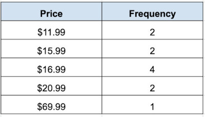
What is the mean price of the trains that Josh is selling?

To answer this question, we simply find the mean (average) by calculating the product of each row. We can do this simply in Excel or Google Sheets by adding a column and multiplying the price (column 1) by the frequency (column 2). We then find the sum of the new product column. We obtain:

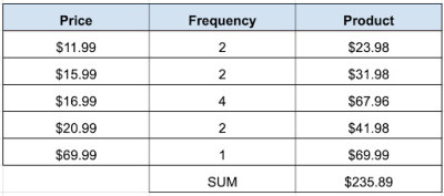
To find the mean, we divide the sum by the total number of trains:  

• $235.89/11 = $21.44 

The mean price of the trains is $21.44.

(You can learn how to find the mean of a data set by using Excel here).

Outliers

Suppose Josh tells a friend that the average price of the trains in his inventory is $21.44. That’s certainly true, but is it an accurate picture of what’s happening here?

If we look a bit closer at Josh’s inventory, we can see that in reality, only one train is selling for more than $21.44. It looks as though Josh has a high valued, possibly rare train that he’s selling for $69.99.

That number is much higher than most of the data. When this happens, we call that number an outlier. An outlier could also be a number that is much lower than the rest of the data.

In statistics, the mean is greatly affected by outliers. An outlier drags the mean in the direction of the outlier. 

Would the same be true of the median? In other words, will the median be affected by the outlier? Let’s look.

Example: Median

What is the median price of the trains that Josh is selling?

We can easily find the median price of the data. Since the table already lists the prices in increasing order, the median is just the middle number. In a data set of 11 numbers, the middle number will occur at the 6th value. Using the frequency column, we can see that the median will be in the third row, $16.99.

The median price of the trains Josh is selling is $16.99.

In this case, the median paints a more accurate picture of the prices of Joshua’s inventory. It summarizes the prices of Josh’s inventory a bit better.

(You can learn more about the differences between mean and median here).

Another question to consider – if we remove the outlier, how are the mean and median affected? We can probably guess that the mean will change significantly! Let’s confirm our hypothesis by removing the outlier from this data set. 

Example: Outlier Removed

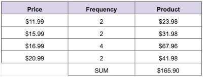
The total number of trains is now 10. So, the new mean after removing the outlier is:

• $165.90/10 = $16.59.

The mean price of each train in the new data set is $16.99.

Now let’s find the median of the new data set. The median of 10 data items is the mean of the two middle numbers.

In this case, the two middle numbers will be the 5th and 6th numbers on the list. Looking at the frequency column, we can see that both the fifth data item and the sixth data item occur in row 3 and have a value of $16.99. 

The median price of each train in the new data set is $16.99. Notice – the median hasn’t changed!

Now let’s compare the effect of the outliers:

Statistic	Original Data Set	New Data Set with Outlier Removed	Change
Mean	$21.44	$16.59	$4.85
Median	$16.99	$16.99	$0

Notice, the mean changed from $21.44 to $16.59, which is a pretty significant difference! The median remained the same, $16.99, in both cases. 

As we can see, something interesting is happening here. The mean is greatly affected by the outlier but the median isn’t.

Another way of saying this is that the median is a resistant statistic  – it resists the temptation to move in the direction of the outlier!

Resistant Statistics don’t change or don’t change too much when there are outliers present in the data.  Resistant statistics aren’t affected by extreme high or low values. The median is a resistant statistic.

Non-Resistant Statistics are affected by outliers or data that is skewed. Non-Resistant statistics are best used with symmetric data. The mean is a non-resistant statistic.

Which statistics are resistant to outliers?

What about other statistics that we’ve learned about? Which ones will be resistant to outliers and which ones will be non-resistant?

Let’s consider the following statistics to see if we can determine if they are resistant or non-resistant.

• Standard Deviation
• Range
• Mode

Standard Deviation

Recall that the standard deviation, denoted by 𝜎, measures the spread of the data. The standard deviation gives us a better idea of how the data is dispersed around the center.

The standard deviation is calculated by finding the squared distances from the mean. Let’s think about whether outliers will affect the standard deviation.

To consider this, it’s helpful to remember that the formula for the standard deviation involves the mean, which implies that the standard deviation will be non-resistant to outliers as well.

As a fun exercise, let’s compare the standard deviation of our two data sets – the prices of the trains including the expensive $69.99 train vs. the prices of the trains without the outlier. We can easily do this on the TI-84 Plus.

Enter the original data from the first table into two columns – the data in one column and the corresponding frequency in the next column. Press Stat, then select Edit (option 1), and press Enter.

Now, enter the train prices into an empty column on screen. If none of your columns are empty, use the arrow key to highlight the column title, then Clear and arrow back down into the column.

Once you’ve finished entering the data into that column, enter the corresponding frequencies in the next column. Also, make a mental note as to which columns you stored the data and their frequencies.

Now, we’re ready to find the standard deviation. Select Stat again, only this time, right arrow to CALC then choose Option 1: 1-Var Stats.

For List: type in the column name. Arrow down and enter the column name for the FreqList (frequencies).

Arrow down to highlight “Calculate” then press Enter. There you have it! You’ll see a list of data.

Now we just need to interpret the data. To find the standard deviation, scroll down to see that the standard deviation 𝜎x is 15.59 (rounded).

Now, let’s delete the outlier from our data and recalculate the standard deviation, following the steps from above.

This time, we get that the standard deviation 𝜎x is $2.87. That is a huge difference from our first value!

The standard deviation decreased by $12.72. The large standard deviation $15.59 suggests that the data for our original table is spread out when in reality there is only 1 data point that is far from the center.

We have 11 data items but that outlier really affected the standard deviation. Since our data is skewed, the standard deviation isn’t a great descriptor of the data.

Once the outlier is removed, that standard deviation drops to $2.87. Now the data is more clustered around the center so the standard deviation is a good descriptive statistic for us.

This confirms that the standard deviation is a non-resistant statistic. It is sensitive to extreme values.

(You can learn how to calculate standard deviation in Excel here).

Range

What about the range? Do we think the range is a resistant or a non-resistant statistic?

Recall that the range is the difference between the maximum value and the minimum value in the data set.

Since an outlier is a value that is either much greater than or much less than the rest of the data, it follows that the outlier will be either the maximum or the minimum value.

Therefore, removing the outlier will greatly affect the range. Let’s calculate the range for both of our data sets in our examples to confirm our theory. 

In our original data set, the maximum value of the train prices is $69.99 and the minimum value is $11.99. The range is the difference 69.99 – 11.99 = 58.00. So, the range of the original data set is $58.

Now, let’s look at our new data set with the outlier removed. The new maximum is $20.99 and the minimum remains unchanged at $11.99. The range is 20.99 – 11.99 = 9.00. Therefore, the range of the new data set is $9. That’s a big difference from the range of $58! 

Conclusion? The range is a non-resistant statistic. It is greatly affected by extreme values.

Mode

What do we think about the mode? Recall that the mode of a data set is the number that occurs the most.

In some cases, there may be no mode or there may be more than one mode. In our example with the trains, the mode of the original set of data is $16.99 since this price occurs 4 times, more frequently than any other value.

In the new data set with the outlier removed, the mode is still $16.99. Therefore, we can conclude that the mode is a resistant statistic. It is not affected by the outlier.

(You can learn how to calculate the mode of a data set in Excel here).

Here is a summary of what we’ve learned so far:

Resistant Statistics	Non-Resistant Statistics
median mode	mean standard deviation range

What can we conclude from our study here? In general, non-resistant statistics like the mean are best used with symmetric data so the statistic won’t be influenced by outliers. Resistant statistics like the median can be used for symmetric and skewed data. 

Are you interested in researching this a bit more? Try to determine if the IQR (Interquartile Range) is a resistant or non-resistant statistic.

---