How To Find Mode In Excel (Plus 5 Helpful Things To Know)

Finding the mode (or “most often seen” value) of a set of numbers helps us to find the most likely outcome in a probability distribution.  Microsoft Excel can find the mode for any set of values you choose as input.

So, how do you find mode in Excel?  To find mode in Excel, use the “MODE” function. The input to the mode function is a range of cells (you can enter multiple cells, rows, columns, or blocks, separating inputs with a comma). For example, the mode of the values in cells A1 to A20 is given by the formula “=MODE(A1:A20)”.

Of course, there can be more than one mode for a data set in some case.  Luckily, Excel also has more specific mode functions (MODE.SNGL and MODE.MULT) to deal with these cases.

In this article, we’ll talk about finding mode in Excel, including how to do it, alternative methods, and when you might use it. We’ll also look at some examples to make the concept clear.

Let’s get started.

How To Find Mode In Excel

The easiest way to find the mode (the most often seen or highest frequency value) in Excel is to use the “MODE” function.  This function can take one or more inputs, separated by commas.

Each input is one or more cells – an input can be:

• a single cell (for example, “A1” would be a single cell)
• a row (for example, “A1:J1” would be a row consisting of 10 cells)
• a column (for example, “A1:A8” would be a column consisting of 8 cells)
• a block of cells (for example, “A1:J8” would be a block of cells consisting of 8 rows and 10 columns, for a total of 8*10 = 80 cells)
• a named range (for example “my_values”, which could denote any set of cells you choose, including an individual cell, a row, a column, or a block of cells)

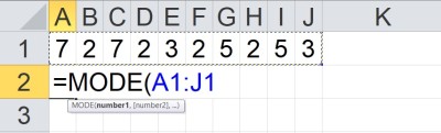
For example, the mode of the values in cells A1 to J1 (a row of 10 cells) would be given by the formula

• =MODE(A1:J1)

You can see an example of this illustrated below.

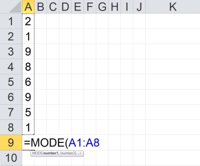
The mode of the values in cells A1 to A8 (a column of 8 cells) would be given by the formula

• =MODE(A1:A8)

You can see an example of this illustrated below.

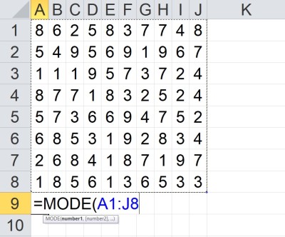
The mode of the values in cells A1 to J8 (a block of 80 cells) would be given by the formula

• =MODE(A1:J8)

You can see an example of this illustrated below.

The mode of the value in cells A1 to A5 and C1 to C5 would be given by the formula

• =MODE(A1:A5, C1:C5)

You can see an example of this illustrated below.

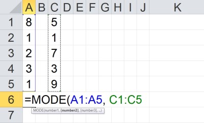
Note that the two inputs (A1:A5 and C1:C5) are separated by a comma.  Each input has a total of 5 cells, for a total of 10 cells as input.

How Is Mode Calculated In Excel? (How Does Excel Find Mode)

MODE returns a single value (the highest frequency value) as an output.  If two or more values are “tied” for highest frequency, then this function returns the smallest (minimum) of those values.

According to Microsoft Support:

“If the data set contains no duplicate data points, MODE returns the #N/A error value.”

https://support.microsoft.com/en-us/office/mode-function-e45192ce-9122-4980-82ed-4bdc34973120

In other words, if the frequency of every value in the data set is 1, the MODE function will return the error #N/A.

Excel needs to take a few steps to calculate the mode of a set of values (cells):

• First, make a list of all the unique values in the data set.
• Next, count how many times each unique value appears (that is, calculate the frequency for each unique value).
• If each value has a frequency of 1, return the “#N/A” error.
• Then, if there are multiple values with the highest frequency, use the minimum of the “tied” values as the mode.  Otherwise, the highest frequency value is the mode.

Note that we can take the mode of any combination of cells, rows, columns, and blocks.  The values don’t need to be in any particular order – the mode function will count the frequency for each value and find the “most often seen” one for us.

Note that MODE.SNGL and MODE.MULT work a little differently on the last step – you can learn more below.

MODE.SNGL vs MODE.MULT In Excel

More recent versions of Excel expand on the MODE function with two specialized functions.  Both take the same inputs as MODE (as described above), but their outputs vary:

• MODE.SNGL returns a single value (the highest frequency value) as an output.  If two or more values are “tied” for highest frequency, then this function returns the smallest (minimum) of those values.
• MODE.MULT returns a vertical array as an output.   This vertical array contains all values of mode. If there is a single mode value, the array contains only one value – but if there are multiple values of mode, then the array contains all of them.

Note that for MODE.MULT to work properly, you must select a column of cells to contain the vertical array, enter the formula (=MODE.MULT(…)), and press “CTRL + SHIFT + ENTER”. This will return the vertical array of modes in the cells you originally selected.

Also note that if there are no repeated values in the data set, both of these functions will return the error #N/A (just as MODE does).

Here are two examples of how to find the mode of a data set in Excel – one using MODE.SNGL and one using MODE.MULT.  We’ll start with MODE.SNGL.

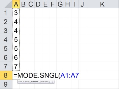
Example 1: Finding The Mode Using MODE.SNGL

Let’s say we want to take the mode of a set of the 7 values shown below:

• {3, 4, 4, 5, 5, 6, 7}

We can see that there are 5 unique values (3, 4, 5, 6, and 7), with counts as shown in the following table:

Value	Frequency (Count)
3	1
4	2*
5	2*
6	1
7	1

This means that both 4 and 5 are tied for the highest frequency (both have a count of 2).

The MODE.SNGL function should take the minimum of these two values (4 and 5) to return 4.  We can verify this below.

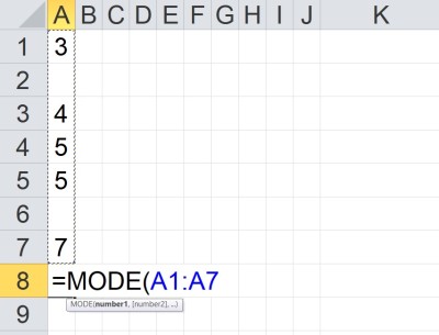
Example 2: Finding The Mode Using MODE.MULT

Let’s say we want to take the mode of a set of the 7 values shown below:

• {3, 4, 4, 5, 5, 6, 7}

We can see that there are 5 unique values (3, 4, 5, 6, and 7), with counts as shown in the following table:

Value	Frequency (Count)
3	1
4	2*
5	2*
6	1
7	1

This means that both 4 and 5 are tied for the highest frequency (both have a count of 2).

The MODE.MULT function should return a vertical array containing both of these values (4 and 5) to return 4.  We can verify this below.

As a reminder: remember that for MODE.MULT to work properly, you must select a column of cells to contain the vertical array, enter the formula (=MODE.MULT(…)), and press “CTRL + SHIFT + ENTER”. This will return the vertical array of modes in the cells you originally selected.

Below, we selected the cells A8 to A9, entered the formula “=MODE.MULT(A1:A7)”, and pressed “CTRL + SHIFT + ENTER”.

Does Mode In Excel Ignore Blank Cells?

Mode in Excel does ignore blanks.  According to Microsoft Support:

“If an array or reference argument contains text, logical values, or empty cells, those values are ignored; however, cells with the value zero are included.”

If you wish to include blank cells in the mode calculation, then you must fill them in with some value (perhaps a value that does not appear in your list and is larger than all other values, so this “filler” value is not calculated to be the mode).

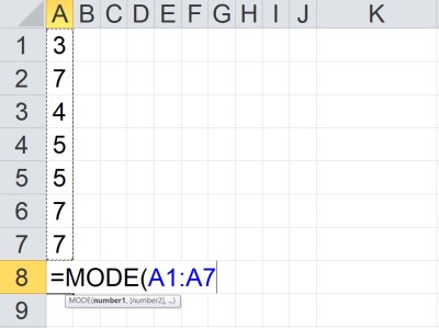
Example: Mode Function Ignores Blank Cells In Excel

If we take the mode of a column of 7 cells in Excel (two of which are blank), the blank cells are ignored (that is, they are not treated as zeroes or any other value).

You can see an example of this below:

However, if we fill in the two blank cells with values of 7, then we get a different mode, as shown below:

What Is The Meaning Of Mode In Excel?

Remember that mode is a measure of center.  It helps us to get an idea of where the “middle” of a data set lies.

Mode tells us the highest frequency value in the data set (that is, the most often seen value).  The mode also tells you the maximum (peak) value on a graph of the data.

A data set can have one, two, three, or more modes. Mode is not the same as mean or median, but they are equal in some cases.

You can learn more about what mode tells you about a data set here.

Why Is Mode Not Working In Excel?

According to Microsoft Support, there are several reasons that the MODE function is not working in Excel:

• One or more of the inputs (cells, rows, columns, blocks, named ranges) contains an error value (such as #N/A, etc.). If this is the case, try checking equations in those input cells to see where the errors are coming from.
• One or more of the inputs (cells, rows, columns, blocks, named ranges) contains text that cannot be translated into a number.
• The data set contains no duplicate data points (that is, the frequency of every data point is 1, and so every number is the most often seen, which means there is no mode).

If the MODE.MULT function is only returning one value when you know that it should be returning 2 or more in a vertical array, remember that for MODE.MULT to work properly, you must:

• select a column of cells to contain the vertical array
• enter the formula (=MODE.MULT(…))
• press “CTRL + SHIFT + ENTER”

This will return the vertical array of modes in the cells you originally selected.

Conclusion

Now you know how to find mode in Excel, as well as the uses of the alternative functions MODE.SNGL and MODE.MULT.

You can learn more about mode and other descriptive statistics here.

You can learn how to find mean in Excel here.

You can learn how to find median in Excel here.

---