
Statistical dispersion helps us to get a handle on a data set by telling us whether its values are close together or far apart. Some measures of statistical dispersion help us to figure out how much variability, volatility, or risk there is in a given data set.
So, what is statistical dispersion? Statistical dispersion tells how spread out the data points in a distribution are. A low dispersion means closely clustered data. A high dispersion means the data is spread far apart. Dispersion can be uniform, random, or clustered, and we measure it with standard deviation, range, & other metrics.
Of course, we must often use a sample standard deviation to measure a population standard deviation, due to the challenge of polling an entire large population.
In this article, we’ll talk about statistical dispersion, what it is, and how we measure it. We’ll also identify the three main types of statistical dispersion and take a look at some examples.
Let’s get started.
What Is Statistical Dispersion?
Statistical dispersion tells us how spread out (dispersed) the data points in a distribution are. A low dispersion means the data is clustered close together, and a high dispersion means the data is spread far out.
For example, we can use various metrics to measure statistical dispersion of the height of humans. Generally, the height of a human runs from 1 foot to 9 feet – the data values are clustered in this range, since nobody is 20, 50, or 100 feet tall.
On the other hand, annual income can range from $0 all the way up to $1 million dollars or more, so the dispersion is high for income.
The lowest possible dispersion for a distribution is when all of the data points have the same value (a constant).
Let’s take a look at some measures of statistical dispersion that can help us to get a handle on how data is spread out.
Measures Of Statistical Dispersion
There are several measures of statistical dispersion that you can use, including:
- Standard Deviation (the square root of variance)
- Range
- Interquartile Range (You can learn how to find quartiles in Excel here).
Let’s take a closer look at each of these in turn, starting with standard deviation.
Standard Deviation
For a data set x1, … , xN, standard deviation has the formula
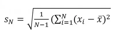
Standard deviation tells us how far, on average, each data point is from the mean:
- A large value for standard deviation means that the data is spread far out, with some of it far away from the mean. That is, on average, a given data point is far from the mean.
- A small value for standard deviation means that the data is clustered near the mean. That is, on average, a given data point is close to the mean.
- A zero value for standard deviation means that all of the data has the same value (which is also the value of the mean). This situation is rare, but it is possible.
Standard deviation tells us about the variability of values in a data set. It is a measure of dispersion, showing how spread out the data points are around the mean. Together with the mean, standard deviation can also indicate percentiles for a normally distributed population.
You can learn about how standard deviation is used in real life in my article here.
Example: Finding The Sample Standard Deviation Of A Data Set
Consider the data set:
- A = {1, 3, 5, 5, 6}
Following the steps above to find the sample standard deviation:
For step 1, we calculate the sample mean. The sample size is n = 5, so:
- Mean = M = (1 + 3 + 5 + 5 + 6) / 5 = 20 / 5 = 4
Now we will use a table to calculate the necessary values for steps 2 and 3:
| Data Value | Value Minus Mean (X-M) | Squared Difference |
|---|---|---|
| 1 | -3 | 9 |
| 3 | -1 | 1 |
| 5 | 1 | 1 |
| 5 | 1 | 1 |
| 6 | 2 | 4 |
from the mean, and squared
differences for the data set.
For step 4, the sum of the square differences (3rd column in the table above) is 9 + 1 + 1 + 1 + 4 = 16.
For step 5, we divide by n – 1. Here n = 5, so n – 1 = 4, and so 16 / (n – 1) = 16 / 4 = 4.
For step 6, we take the square root of 4 to get 2.
So, the sample standard deviation is 2.
Range
The range of a data set is the difference between the maximum (largest value) and minimum (smallest value):
- Range = Maximum – Minimum
The range is the minimum width of the interval that contains every data point in the distribution – that is, the interval [Minimum, Maximum].
However, using the range of a data set to tell us about the spread of values has some disadvantages:
- Range only takes into account two data values from the set: the maximum and the minimum. The rest of the data values are ignored.
- Range does not tell us anything about how far the average data point is from the mean. In fact, range does not take the mean into account at all.
- Range is highly susceptible to outliers, regardless of sample size. Whenever the minimum or maximum value of the data set changes, so does the range – possibly in a big way.
Standard deviation, on the other hand, takes into account all data values from the set, including the maximum and minimum.
Example: Calculating The Range Of A Data Set
Consider the data set:
- A = {1, 3, 5, 5, 6}
To find the range, we follow these steps:
- Find the minimum data value (here, Minimum = 1).
- Find the maximum data value (here, Maximum = 6).
- Find the difference between them to get the range (here, Maximum – Minimum = 6 – 1 = 5).
Interquartile Range
Interquartile range (IQR) is sometimes called the “Middle 50%”. It is similar to the range, but instead of taking the difference of the maximum and minimum, we take the difference of Q3 (third quartile) and Q1 (first quartile):
- IQR = Q3 – Q1
Recall that for a data set:
- Q1, the first quartile, is the 25th percentile of the distribution. It is the value that is greater than or equal to 25% of the data values (or less than or equal to 75% of the data values).
- Q2, the second quartile (median), is the 50th percentile of the distribution. It is the value that is greater than or equal to 50% of the data values (or less than or equal to 50% of the data values).
- Q3, the third quartile, is the 75th percentile of the distribution. It is the value that is greater than or equal to 75% of the data values (or less than or equal to 25% of the data values).
So, when we take the difference Q3 – Q1, we get the 75th percentile minus the 25th percentile, leaving us the “spread” of the middle 50% of the data. We are effectively leaving out the top 25% and bottom 25% of the data values, which should rid us of most or all outliers.
Example: Calculating The Interquartile Range Of A Data Set
Consider the data set:
- A = {1, 2, 3, 3, 5, 6, 6, 8, 9, 9, 11, 12}
There are 12 data points, and the median (middle) value is 6, so Q2 = 6.
The bottom 50% of the data is the subset {1, 2, 3, 3, 5, 6}. There are 6 data points, and the median (middle) value is 3, so Q1 = 3.
The top 50% of the data is the subset {6, 8, 9, 9, 11, 12}. There are 6 data points, and the median (middle) value is 9, so Q3 = 9.
Then the interquartile range (IQR) is:
- IQR = Q3 – Q1
- IQR = 9 – 3
- IQR = 6
What Are The Three Types Of Dispersion?
When examining a data distribution, the three types of dispersion are:
- Uniform Dispersion – the data points are spaced or distributed evenly.
- Random Dispersion – the data points are distributed in a way that is difficult to predict, with no discernible pattern.
- Clumped Dispersion – the data points are clustered in groups.
Let’s take a closer look at each one, starting with uniform dispersion.
Uniform Dispersion
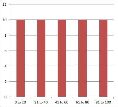
In a uniform dispersion, the data points are spaced evenly. The occurrence of each data value has the same frequency.
Example: Uniform Dispersion
Let’s say that we survey a group of 50 people to find out where they fall in the following five age ranges:
- 0 to 20 years
- 21 to 40 years
- 41 to 60 years
- 61 to 80 years
- 81 to 100 years
After the survey, we find that there are exactly 10 people in each age range. This is an example of uniform dispersion, which you can see in the graph below:
Random Dispersion
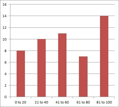
In a random dispersion, the data points are spaced in a way that does not have a pattern.
Example: Random Dispersion
Let’s say that we survey a group of 50 people to find out where they fall in the following five age ranges:
- 0 to 20 years
- 21 to 40 years
- 41 to 60 years
- 61 to 80 years
- 81 to 100 years
After the survey, we find that the counts are 8, 10, 11, 7, and 14. This is an example of random dispersion, which you can see in the graph below:
Clumped Dispersion
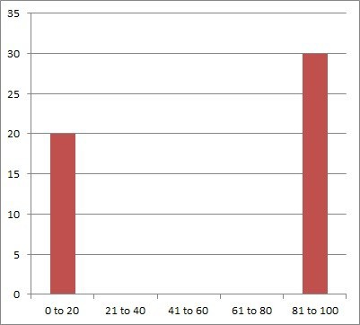
In a random dispersion, the data points are spaced close together, possibly in different groups.
Example: Clumped Dispersion
Let’s say that we survey a group of 50 people to find out where they fall in the following five age ranges:
- 0 to 20 years
- 21 to 40 years
- 41 to 60 years
- 61 to 80 years
- 81 to 100 years
After the survey, we find that there are exactly 20 people in the youngest range and 30 people in the oldest age range. This is an example of clumped dispersion, which you can see in the graph below:
Conclusion
Now you know what statistical dispersion is and how to measure it. You also know the three main types of statistical dispersion and what each one looks like.
You might also want to learn about the concept of a skewed distribution (find out more here).
Some statistics are resistant to outliers, while others are not – you can learn more here.
You can learn more about data literacy in my article here.
You can learn how to calculate percentiles in Excel here.
I hope you found this article helpful. If so, please share it with someone who can use the information.
Don’t forget to subscribe to my YouTube channel & get updates on new math videos!
~Jonathon