Finding Correlation Coefficients In Excel (5 Helpful Tips)

Finding the correlation coefficient for two groups of numbers helps us to figure out how the data sets are related – and may also help us to make predictions.  Microsoft Excel can find the correlation coefficient for any two sets of values you choose as input.

So, how do you find a correlation coefficient in Excel?  To find correlation coefficients, use Excel’s CORREL function. The CORREL function’s input is two arrays (rows, columns, blocks) of cells (arrays must be the same size). For example, the formula “=CORREL(A1:A8, B1:B8)” gives the correlation coefficient of the values in cells A1 to A8 and B1 to B8.

Of course, a correlation coefficient can be positive, negative, or zero (a value between -1 and 1).  An absolute value closer to 1 means a strong correlation.

In this article, we’ll talk about finding correlation coefficients in Excel and how to interpret them.  We’ll also look at several examples with positive and negative correlation coefficients.

Let’s get started.

How To Calculate Correlation Coefficient In Excel (R-Value In Excel)

The easiest way to find the correlation coefficient (which is one way to measure the relationship between two variables or data sets) in Excel is to use the “CORREL” function.

This function takes two separate array inputs, which are separated by commas.  Note that the arrays must have the same “size” (number of cells).

Also note that any text, logical values, or empty cells are ignored – only numbers are used to calculate the correlation coefficient.

Each input array contains at least two cells – an input can be:

• a single cell (for example, “A1” would be a single cell)
• a row (for example, “A1:J1” would be a row consisting of 10 cells)
• a column (for example, “A1:A8” would be a column consisting of 8 cells)
• a block of cells (for example, “A1:J8” would be a block of cells consisting of 8 rows and 10 columns, for a total of 8*10 = 80 cells)
• a named range (for example “my_values”, which could denote any set of cells you choose, including an individual cell, a row, a column, or a block of cells)

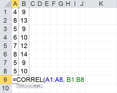
For example, for two sets of data in column form (first column consisting of the cells A1:A8, and the second column consisting of the cells B1:B8), the formula for calculating the correlation coefficient would be:

• “=CORREL(A1:A8, B1:B8)”

You can see how this looks in Excel below:

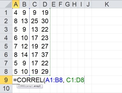
Similarly, for two sets of data in cells A1:B8 and C1:D8, the formula for calculating the correlation coefficient would be:

• “=CORREL(A1:B8, C1:D8)”

You can see how this looks in Excel below:

Note that in these examples, the “size” (number of cells in the array) for both data sets is the same.

Remember that the order of the values matters.  Changing the order of values for one data set but not the other will change the correlation coefficient.

The reason is that each “point” on the graph represents a pair of values: one from each data set.  If the order of the values in a data set changes, then the points on the graph change, and the correlation coefficient (and line of best fit) also change.

You can learn more about line of best fit (and scatter plots) here.

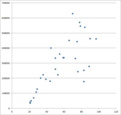
How To Find The Correlation Coefficient On A Scatter Plot In Excel

If you already have a scatter plot in Excel created from two data sets, then you can find the correlation coefficient as follows:

• First, click on the scatter plot you created.
• Next, right-click on one of the data points in the scatter plot.
• Then, select the “Add Trendline” option.
• Now, select the “Linear” radio button in the dialog.
• Next, check the “Display R-squared value on chart” box.
• Finally, take the square root of the R-squared (R²) value that is displayed.

You can see some screenshots below.

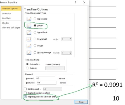
For example, if the displayed R² value on the scatter plot is 0.81, then |R| = 0.9 (that is, the correlation coefficient is 0.9), since:

• R² = 0.81
• √(R²) = √(0.81)
• |R| = 0.9

To find the sign of R, you must look at the slope of the line of best fit. If the slope is positive, then R is positive; if the slope is negative, then R is negative.

This is a fairly strong positive correlation, since the highest possible correlation coefficient is 1.

What Is The Correlation Coefficient In Excel? (Meaning Of Correlation Coefficient)

The correlation coefficient (R-value) in Excel is one measure we can use to find out how strong the relationship is between two data sets (variables).

The correlation coefficient R always has a value between -1 and 1, meaning -1 <= R <= 1.   We can also say that 0 <= |R| <= 1.

• If |R| has a value of 0, then there is no correlation between the variables.
• If |R| has a value close to 0, then there is a weak correlation between the variables.
• If |R| has a value close to 1, then there is a strong correlation between the variables.
• If R is positive, then one variable tends to increase as the other increases.
• If R is negative, then one variable tends to decrease as the other increases.

Example 1: Finding Correlation Coefficients In Excel (Positive Correlation Coefficient)

Let’s say that we have the following table of data in Excel (split into two separate columns, with one data set per column):

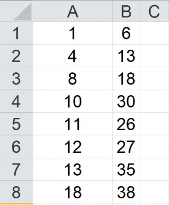
To find the correlation coefficient, we use the CORREL function.  The input ranges are A1:A8 and B1:B18, which gives us a formula of:

• =CORREL(A1:A8, B1:B8)

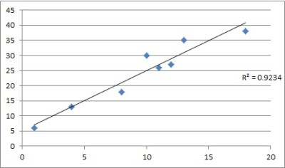
The resulting correlation coefficient is positive (with a value of approximately 0.96).  This is a fairly strong positive correlation between the two data sets (meaning that the values in both data sets tend to increase or decrease together).

This implies that we might have some success in predicting the values of one variable, given values of the other.  However, remember that correlation does not imply causation (this means we don’t necessarily know which variable is independent and which is dependent).

We can confirm the positive correlation by graphing a scatterplot of the points in the data table and drawing the line of best fit (which has a positive slope).

Example 2: Finding Correlation Coefficients In Excel (Negative Correlation Coefficient)

Let’s say that we have the following table of data in Excel (split into two separate columns, with one data set per column):

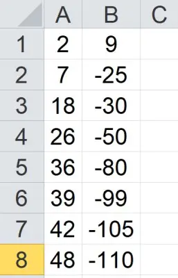
To find the correlation coefficient, we use the CORREL function.  The input ranges are A1:A8 and B1:B8, which gives us a formula of:

• =CORREL(A1:A8, B1:B8)

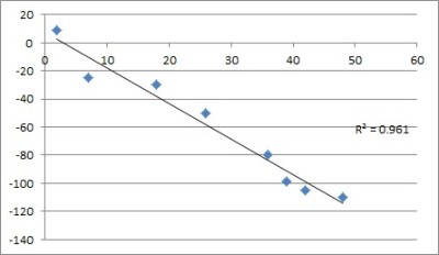
The resulting correlation coefficient is negative (with a value of -0.98).  This is a fairly strong negative correlation between the two data sets (meaning that as the values in one data increase, the value sin the other data set tend to decrease).

This implies that we might have some success in predicting the values of one variable, given values of the other.  However, remember that correlation does not imply causation (this means we don’t necessarily know which variable is independent and which is dependent).

We can confirm the negative correlation by graphing a scatterplot of the points in the data table and drawing the line of best fit (which has a positive slope).

Example 3: Finding Correlation Coefficients In Excel (Near Zero Correlation Coefficient)

Let’s say that we have the following table of data in Excel (split into two separate columns, with one data set per column):

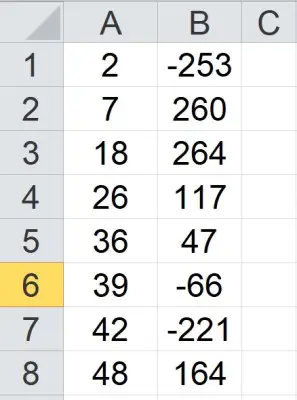
To find the correlation coefficient, we use the CORREL function.  The input ranges are A1:A8 and B1:B8, which gives us a formula of:

• =CORREL(A1:A8, B1:B8)

The resulting correlation coefficient is negative, but close to zero (with a value of -0.07).  This is a fairly weak negative correlation between the two data sets (meaning that it is difficult to make the case for a strong connection between the values in the data sets).

This implies that we might not have much success in predicting the values of one variable, given values of the other.

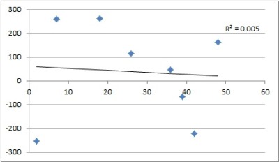
We can confirm the weak correlation by graphing a scatterplot of the points in the data table and drawing the line of best fit (which has a slightly negative slope).

Excel CORREL Function #DIV/0 (Divide By Zero Error)

According to Microsoft Support, the CORREL function will display the #DIV/0 error in a couple of cases:

• One or both input arrays are empty.
• The standard deviation of one or both input arrays is zero (this can happen if there is only one value for either array, or if all values in an array are the same).

Excel CORREL Function #N/A (N/A Error)

According to Microsoft Support, the CORREL function will display the #N/A error if:

• The two input arrays have a different number of data points (cell counts for the two arrays are not the same).

Conclusion

Now you know how to find correlation coefficients in Excel.  You also know what this measure means and how it can tell you about the relationship between two data sets.

You can learn how to find mean in Excel here.

You can learn how to find median in Excel here.

You can learn how to find mode in Excel here.

---