
You may know how to calculate the second derivative of a function, but do you know what it means? The second derivative of a function gives us lots of information about the graph and what it looks like, especially when considered with the first derivative.
So, what does second derivative tell you? The second derivative tells you concavity & inflection points of a function’s graph. With the first derivative, it tells us the shape of a graph. The second derivative is the derivative of the first derivative. In physics, the second derivative of position is acceleration (derivative of velocity).
Of course, the second derivative is not the highest derivative of a function that we can take. We can take third, fourth, and fifth derivatives – as long as the previous derivative is differentiable.
In this article, we’ll talk about the second derivative and what it tells you about a function and its graph. We’ll also look at some examples to make the concepts clear.
Let’s get started.
Hey! If you need to learn more about second derivatives and other math concepts for physics, check out this course:
Advanced Math For Physics: A Complete Self-Study Course
What Is The Second Derivative Of A Function?
The second derivative of a function f(x) is the derivative of the derivative of f(x). In other notation:
- f(x) is the original function
- f’(x) is the derivative of f’(x)
- f’’(x) is the second derivative of f(x) and the first derivative of f’(x)
Remember that the derivative of a function tells us the slope of the tangent line at a given point. That is, the first derivative of a function tells us how the function is changing.
What Does Second Derivative Tell You?
The second derivative f’’(x) tells you how fast the first derivative f’(x) is changing. However, there is a lot more that the second derivative can tell us, such as:
- Concavity of the graph of the function (which way the function opens: up or down)
- Inflection points of the graph of the function (where concavity changes)
- Shape of the graph of the function (together with first derivative)
- Rate of change of the first derivative (the derivative of the first derivative)
- Acceleration of an object (rate of change of velocity: is the object speeding up or slowing down?)

Let’s take a closer look at each of these, along with some examples.
Second Derivative For Concavity Of The Graph Of A Function
The sign of the second derivative f’’(x) tells us the concavity of the graph of the function f(x). Essentially, this tells us whether the function opens upward (like a cup) or downward (like a dome).
Here is what you need to know about the second derivative as it relates to concavity of a function:
- A function f(x) is concave (or concave down) if the 2nd derivative f’’(x) is negative, with f’’(x) < 0. Graphically, a concave function opens downward, and water poured onto the curve would roll off.
- A function f(x) is convex (or concave up) if f’’(x) is positive, with f’’(x) > 0. Graphically, a convex function opens upward, and water poured onto the curve would fill it.
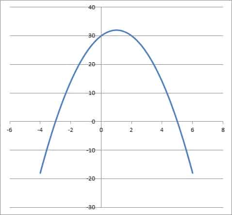
Here is the graph of a concave (concave down) function:
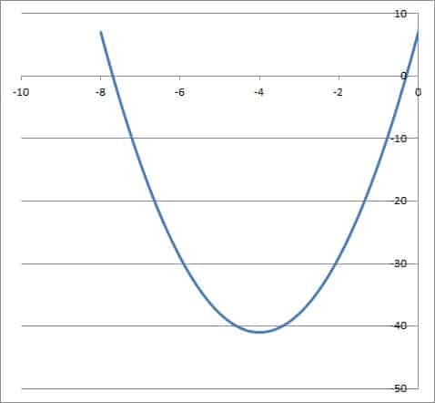
Here is the graph of a convex (concave up) function:
Let’s look at some examples to see if we can find the concavity of some functions.
Example 1: Finding the Concavity of f(x) = x2
Consider the function f(x) = x2.
The first derivative is f’(x) = 2x, by the power rule.
The second derivative is f’’(x) = 2, again by the power rule.
Since 2 is always positive, we have f’’(x) > 0 for all values of x. This means that f(x) is convex (concave up) for all values of x, and it opens upward. (using the Second Derivative Test)
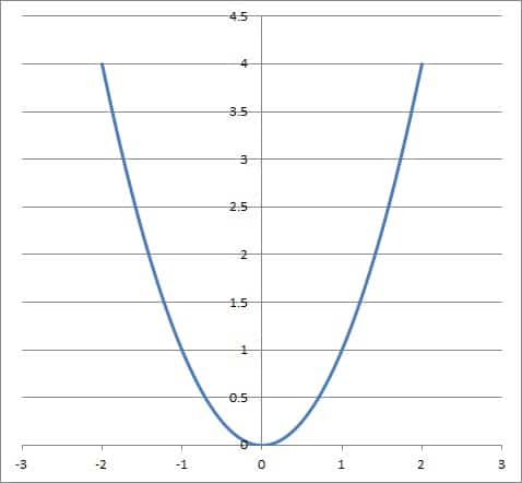
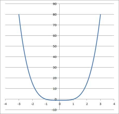
You can see the graph of f(x) = x2 below.
Example 2: Finding the Concavity of f(x) = x3
Consider the function f(x) = x3.
The first derivative is f’(x) = 3x2, by the power rule.
The second derivative is f’’(x) = 6x, again by the power rule.
Since 6x is positive for x > 0, we have f’’(x) > 0 for all positive values of x. This means that f(x) is convex (concave up) for all positive values of x, and it opens upward on the interval x > 0.
Since 6x is negative for x < 0, we have f’’(x) < 0 for all negative values of x. This means that f(x) is concave (concave down) for all negative values of x, and it opens downward on the interval x < 0.
At x = 0, we have f’’(x) = 6x = 6(0) = 0, which means that f(x) is neither convex nor concave at x = 0. This means x = 0 is a possible inflection point for f(x) = x3 (more on this later).
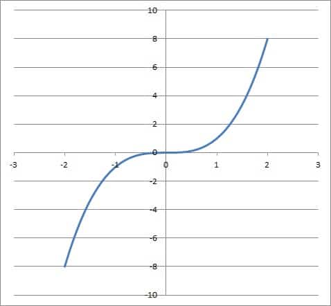
You can see the graph of f(x) = x3 below.
Second Derivative For Inflection Points Of The Graph Of A Function
Now that we know how to find the concavity of a function f(x), we can also find any inflection points that may exist (note that some functions have no inflection point).
An inflection point of a function f(x) is a point where the concavity changes (from positive to negative or from negative to positive). By definition, the second derivative of f(x) will be zero at an inflection point (so f’’(x) = 0).
Let’s look at some examples to see if we can find the inflection points of some functions.
Example 1: Finding The Inflection Points Of f(x) = x3 – 6x2 + 7x – 5
Let’s say we want to find the inflection points of f(x) = x3 – 6x2 + 7x – 5.
The first derivative is f’(x) = 3x2 – 12x + 7, by the power rule.
The second derivative is f’’(x) = 6x – 12, again by the power rule.
We look for a point where f’’(x) = 0 to find a possible inflection point:
- f’’(x) = 0 [this is necessary, but not sufficient, for an inflection point]
- 6x – 12 = 0
- 6x = 12
- x = 2
So the point x = 2 is a possible inflection point of f(x). To confirm, we must verify that the sign of f’’(x) changes at x = 2.
To do this, we will pick two values of x: one that is less than 2, and one that is more than 2. Then, we will evaluate f’’(x) at both of these x values and compare the signs.
Let’s choose x = 1 (for x < 2) and x = 3 (for x > 2).
At x = 1, we have:
- f’’(x) = 6x – 12
- f’’(1) = 6(1) – 12
- f’’(1) = -6
- f’’(1) < 0
At x = 3, we have:
- f’’(x) = 6x – 12
- f’’(3) = 6(3) – 12
- f’’(1) = 6
- f’’(1) > 0
So f’’(x) is negative to the left of x = 2 and positive to the right of x = 2. This means that f’’(x) changes signs at x = 2, and thus it changes concavity at x = 2.
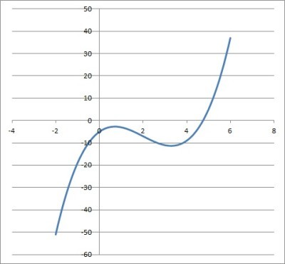
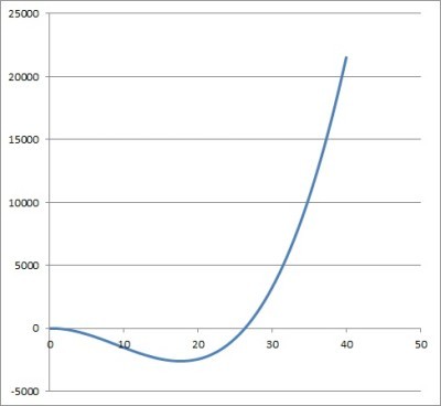
So, x = 2 is an inflection point of f(x) = x3 – 6x2 + 7x – 5, which we can see in the graph below.
Example 2: Finding The Inflection Points Of f(x) = x4
Consider the function f(x) = x4 – 1.
The first derivative is f’(x) = 4x3, by the power rule.
The second derivative is f’’(x) = 12x2, again by the power rule.
We look for a point where f’’(x) = 0 to find a possible inflection point:
- f’’(x) = 0 [this is necessary, but not sufficient, for an inflection point]
- 12x2 = 0
- x2 = 0
- x = 0
So the point x = 0 is a possible inflection point of f(x). However, we can show that f’’(x) does not change signs.
First, we know that x2 >= 0 for all real values of x.
It follows that 6x2 >= 0 for all real values of x.
Then f’’(x) >= 0 for all real values of x.
Since f’’(x) is never negative, it can never change signs. So, the concavity of f(x) can never change, and this function has no inflection point, as we can see in the graph below.
Second Derivative For The Shape Of The Graph Of A Function
The second derivative of a function can also tell us the shape of a function f(x) if we also consider the first derivative.
The following table shows the possible combinations of signs of f’(x) and f’’(x) and what they tell us:
| Sign of f'(x) | Sign of f”(x) | Function Behavior |
|---|---|---|
| – | – | Decreasing; Concave |
| – | 0 | Decreasing; Possible Inflection Point |
| – | + | Decreasing; Convex |
| 0 | – | Possible local extreme; Concave |
| 0 | 0 | Possible local extreme; Possible Inflection Point |
| 0 | + | Possible local extreme; Convex |
| + | – | Increasing; Concave |
| + | 0 | Increasing; Possible Inflection Point |
| + | + | Increasing; Convex |
of a function f(x) based on the
signs of f'(x) and f”(x) [the first
and second derivatives of f(x)].
Let’s look at an example to see how this works in practice.
Example: Finding the shape of f(x) = x3 – 12x2 + 36x – 24.
Consider the function f(x) = x3 – 12x2 + 36x – 24.
The first derivative is f’(x) = 3x2 – 24x + 36, by the power rule.
The second derivative is f’’(x) = 6x – 24, again by the power rule.
The first derivative is zero when:
- f’(x) = 0
- 3x2 – 24x + 36 = 0
- 3(x2 – 8x + 12) = 0
- 3(x – 2)(x – 6) = 0
So x = 2 and x = 6 are values where f’(x) = 0.
The second derivative is zero when:
- f’’(x) = 0
- 6x – 24 = 0
- 6(x – 4) = 0
So x = 4 is the value where f’’(x) = 0.
The following table shows intervals with various signs for f’(x) and f’’(x):
| Interval | Sign of f'(x) | Sign of f”(x) |
|---|---|---|
| x < 2 | + | – |
| x = 2 | 0 | – |
| (2, 4) | – | – |
| x = 4 | – | 0 |
| (4, 6) | – | + |
| x = 6 | 0 | + |
| x > 6 | + | + |
This tells us that the function f(x) is:
- Concave down and increasing when x < 2.
- Concave down and a local maximum when x = 2.
- Concave down and decreasing when 2 < x < 4.
- An inflection point and decreasing when x = 4.
- Concave up and decreasing when 4 < x < 6.
- Concave up and a local minimum when x = 6.
- Concave up and increasing when x > 6.
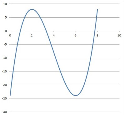
We can verify this with the graph below.
Second Derivative For Rate Of Change Of First Derivative
The second derivative is the derivative of the first derivative. So, f’’(x) tells us how fast f’(x) is changing at a given point.
We can use this idea in business to figure out when a company is growing its revenue, how fast revenue is growing, and whether the growth is slowing down.
Example: First and Second Derivatives For Company Profit
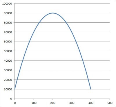
Let’s say that a company has a profit function given by f(x) = -2x2 + 800x + 10,000, where x is the number of items produced and sold.
The first derivative is f’(x) = -4x + 800, by the power rule. This function tells us how the profit is changing: when it is positive, the company’s profit is increasing.
The second derivative is f’’(x) = -4, again by the power rule. This function tells us if the growth rate of profit is slowing down or speeding up.
We know that f’(x) = 0 when:
- f’(x) = 0
- -4x + 800 = 0
- -4x = -800
- x = 200
This tells us that:
- For any value of x < 200, f’(x) is positive and profit is growing for each additional item produced and sold.
- At x = 200, the profit growth stops, since f’(x) = 0.
- For any value of x > 200, f’(x) is negative and profit is declining for each additional item produced and sold (this could be due to increased cost of acquiring rare parts or materials above a certain threshold).
Let’s analyze a particular production level: x = 100.
At x = 100 we have a profit of:
- f(x) = -2x2 + 800x + 10,000
- f(100) = -2(100)2 + 800(100) + 10,000
- f(100) = =2(10,000) + 80,000 + 10,000
- f(100) = -20,000 + 90,000
- f(100) = 70,000
So company profits are $70,000 at a production level of x = 100. Does it make sense to produce more?
At x = 100, the change in profit is:
- f’(x) = -4x + 800
- f’(100) = -4(100) + 800
- f’(100) = -400 + 800
- f’(100) = 400
So company profits grow by $400 if we produce an extra item after x = 100 have been made.
The last question is, how does increased production change the growth in profit?
At x = 100, the second derivative of profit is:
- f’’(x) = -4
- f’’(100) = -4
So every time we produce an extra item, the extra profit we receive decreases by $4. So there is less increase in profit as we increase our production.
Second Derivative For Acceleration Of An Object
Remember that if f(x) is the position function of an object, then f’(x) is the velocity of the object, and f’’(x) is the acceleration of the object.
So, the second derivative of an object’s position function tells us its acceleration.
Let’s see an example.
Example: Using The Second Derivative To Find Acceleration Of An Object
Let’s say that the position of an object is given by the function f(t) = t3 – 27t2 + 18t – 9, where t is the time in seconds (starting at t = 0).
The first derivative is f’(t) = 3t2 – 54t + 18, by the power rule.
The second derivative is f’’(t) = 6t – 54, again by the power rule.
So the acceleration of the object at time t is given by f’’(t).
The acceleration (second derivative) is zero when:
- f’’(t) = 0
- 6t – 54 = 0
- 6(t – 9) = 0
So t = 9 is the value where f’’(t) = 0.
For any value of t greater than 9, f’’(t) is positive (positive acceleration). For example:
- f’’(1) = 6(1 – 9) = 6(-8) = -48 < 0
For any value of t less than 9, f’’(t) is negative (negative acceleration). For example:
- f’’(10) = 6(10 – 9) = 6(1) = 6 > 0
This means that t = 9 is an inflection point of the position function f(t), as we can see in the graph below.
Conclusion
Now you know what the second derivative tells you and what it is. You also have some examples of how it is used to give us more information about a function and its shape.
You can learn how to graph a function from its derivative here.
You can learn about when a function is onto (maps onto the entire codomain) in my article here.
You can learn about how to use derivatives and graphs to find function maximums here.
I hope you found this article helpful. If so, please share it with someone who can use the information.
Don’t forget to subscribe to my YouTube channel & get updates on new math videos!
~Jonathon