What Is The Central Limit Theorem? (3 Key Ideas To Grasp)

In statistics, we want to consider many members of a population at once, as a whole (rather than only one or a few members). When we take a large enough sample from a population, the central limit theorem applies to the data.

So, what is the central limit theorem? The central limit theorem tells us that the sum of “enough” independent random variables starts to look like a normal distribution (even if the variables are not from a normal distribution!) The central limit theorem allows us to use normal distributions for large samples from other distributions.

For example, a single six-sided die roll has a uniform distribution. However, if we add up enough die rolls, we get something that starts to look a lot like a normal distribution.

In this article, we’ll talk about what the central limit theorem is and when we can apply it. We’ll also look at some examples to see this concept in action.

Let’s get started.

What Is The Central Limit Theorem?

The central limit theorem states that:

“For a population with mean M and standard deviation S, the sampling distribution of the mean is approximately normal, with mean M and standard deviation S/√N*.”
*N is the sample size

The beautiful thing about the central limit theorem is that it applies to a population whether or not it is normally distributed.

uniform distribution with zero variance — As long as the sample size is large enough, the Central Limit Theorem applies to independent random samples from a population, even if the population is not normally distributed.

However, for a population that is not normally distributed, the sample size N must be “large enough”, which usually means N >= 30 data points (unless the population is highly skewed).

What Are The Conditions Of The Central Limit Theorem?

The central limit theorem is useful in many contexts. However, we can only apply the theorem if certain things hold true.

The conditions of the central limit theorem include:

Independence – the random variables we are examining should be independent. This means that the value of one variable does not affect another. For example, when you roll two dice and sum them, the value of one die does not affect the value of the other die. To put it another way, the samples we take from the population should be independent (generally, we should choose samples with replacement to ensure this).
Random Sampling – the samples taken from the population should be random. This means no bias towards a specific subset of the population. For example, a sample of elementary school students would not be a random sample from the population of a large city, since their ages will all be between 6 and 10.

Sufficiently large sample size – the sample size must be “large enough” so that the sampling distribution closely approximates a normal distribution. Often, sample size of N >= 30 is cited as “large enough” for independent random variables that are not normal. However, you may need a larger sample size for highly skewed distributions.
Known Parameter Values – we need to know the mean M and the standard deviation S of the distribution to find the mean and standard deviation of the sampling distribution. The standard deviation S must be finite, or else the central limit theorem does not apply.

sample standard deviation 3 (data & value) 2nd — Generally, if the population is not normally distributed, the sample size must be “large enough” to apply the Central Limit Theorem. This means a sample size of at least N >= 30 (or larger if the data is highly skewed).

What Does The Central Limit Theorem Apply To?

The central limit theorem applies to samples from populations that might not be normally distributed. As mentioned above, the random variables must be independent (and samples must be random).

If the population is not normal, then the sample size N must be at least 30.

right skewed distribution positively skewed 2 — This data is not normally distributed, but the Central Limit Theorem will allow us to apply a normal distribution to the sampling distribution.

If the sample size is less than 30, then a normal distribution might not be a good approximation for the sampling distribution.

Does The Central Limit Theorem Apply To All Distributions?

The central limit theorem does not apply to all distributions.

For example, the central limit theorem does not apply to distributions with:

Unbounded standard deviation – in this case, we cannot apply the central limit theorem.
Zero standard deviation – in this case, a sample from the population will have no variability (all of the data points will have the same value, equal to the mean, and every sample mean will be equal to the population mean). Remember: a distribution with zero standard deviation cannot be normal.

Does The Central Limit Theorem Apply To Discrete Random Variables?

The central limit theorem does apply to discrete random variables – as long as the conditions mentioned earlier are met.

You can see an example of the central limit theorem applied to discrete random variables (6-sided dice rolls) below.

Note: the central limit theorem also applies to continuous random variables (again, the conditions mentioned earlier must be met).

Why Is The Central Limit Theorem Important In Statistics?

The Central Limit Theorem is important in statistics because it allows us to use a familiar and widely-used distribution (the normal distribution) to study populations that may or may not be normally distributed.

standard-normal-distribution — The Central Limit Theorem allows us to use the normal distribution for populations that might not be normally distributed.

We do this by taking repeated samples (as long as they are independent random samples) and studying the sampling distribution of the means.

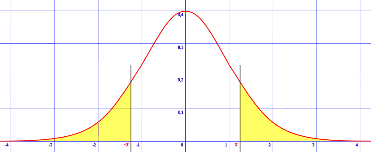
Remember: if we have a normal distribution, we can normalize the variable X with the formula

Z = (X – M)/S

where M is the mean, S is the standard deviation, and Z is a standard normal variable with mean 0 and standard deviation 1.

Once we normalize a variable, we can use a standard normal table to find the probability that the mean of a sample will be greater than a value (or less than a value, or between two values).

For example, we can use the “68-95-99.7 rule” if we know the mean and standard deviation for a normal distribution. Roughly, this rule states that:

68% of the population lies within one standard deviation of the mean
95% of the population lies within two standard deviations of the mean

99.7% of the population lies within three standard deviations of the mean

So, if we have a normal distribution with mean 50 and standard deviation 10, then:

68% of the population lies within one standard deviation of the mean, or in the interval [40, 60].

95% of the population lies within two standard deviations of the mean, or in the interval [30, 70].
99.7% of the population lies within three standard deviations of the mean, or in the interval [20, 80].

normal-distribution-curve — The normal distribution tells us that 68% of data points are within 1 standard deviation of the mean (in either direction), 27% are between 1 and 2 standard deviations from the mean (in either direction), and 4.7% are between 2 and 3 standard deviations from the mean (in either direction). This leaves only 0.3% of the population that is more than 3 standard deviations away from the mean.

When Can You Use The Central Limit Theorem?

You can use the central limit theorem if you have independent random samples from a population and you want to examine the sampling distribution.

By extension, you can also use the central limit theorem when examining the sum or average of independent random variables (even if those variables are not normal).

Example: Using The Central Limit Theorem For A Discrete Random Variable (Average Of N 6-Sided Dice Rolls)

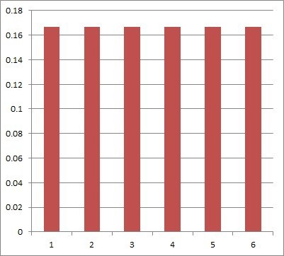
A 6-sided dice roll is a discrete random variable. Assuming the die is fair (not loaded or weighted), the probability distribution is uniform, with a probability of 1/6 for each of the values 1, 2, 3, 4, 5, and 6 (as you can see in the diagram below).

uniform distribution die roll six sided dice — This graph shows the probability distribution for a fair six-sided die. There is a 1/6 chance to roll each of the outcomes 1 through 6.

When we add up the faces on multiple dice and divide by the number of dice, we get an average for N dice. The result approaches a normal distribution – with the same mean as for rolling one die (namely, 3.5), but with much less variation (smaller standard deviation).

For the average of two fair six-sided dice, we get a distribution that is not uniform anymore. The table below shows the possible outcomes of rolling two dice.

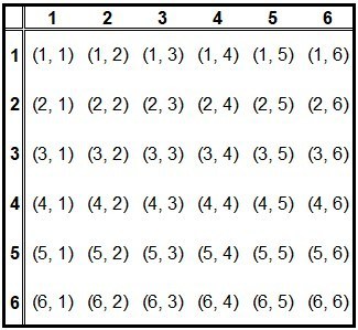
probability table sum of two 6 sided dice (SHOWING ORDERED PAIRS) — This is the table of outcomes for rolling two six-sided dice. To get the sums, we add up the two values in parentheses. There is only one way to get a sum of 2 (1 + 1 = 2, from the top left corner). However, there are 6 different ways to get a sum of 7.

Note that there is only one way to get an average of exactly 1: by rolling “snake eyes” (two ones), summing them to get 2, and dividing by 2 to get 1. However, there are 7 ways to get an average of exactly 3.5:

Roll a 1 on the first die and a 6 on the second, for a total of 7 and an average of 3.5.

Roll a 2 on the first die and a 5 on the second, for a total of 7 and an average of 3.5.
Roll a 3 on the first die and a 4 on the second, for a total of 7 and an average of 3.5.
Roll a 4 on the first die and a 3 on the second, for a total of 7 and an average of 3.5.

Roll a 5 on the first die and a 2 on the second, for a total of 7 and an average of 3.5.
Roll a 6 on the first die and a 1 on the second, for a total of 7 and an average of 3.5.

Note that the graph of the average of two dice is starting to look a little more like a normal distribution (see below).

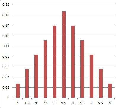
normal shaped distribution die roll average of two six sided dice — This graph shows the probability distribution for the average of two six-sided dice. There is a 1/36 chance to roll an average of 1, but a 1/6 chance to roll an average of 3.5 (the same as the expected value for 1 die).

So the mean for rolling two dice is the same as the mean for rolling one dice (3.5). However, there is more chance of rolling an average closer to 3.5 (meaning a lower variance or standard deviation).

For the average of three fair six-sided dice, we get a graph that looks even more like a normal distribution:

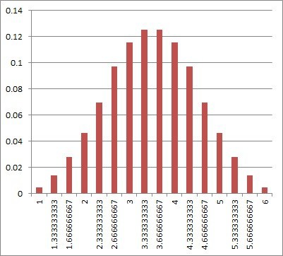
normal shaped distribution die roll average of three six sided dice — This graph shows the probability distribution for the average of three six-sided dice. There is a 1/216 chance to roll an average of 1 (or to roll an average of 6). The expected value is still 3.5 (the same as the expected value for 1 die or 2 dice).

In that case, the probability of rolling an average of exactly 1 is 1/216 (1/6 to the third power). We would have to roll three 1’s on three dice to get an average of 1 – there is not other way to do it.

As we continue to increase the number of dice, the distribution approaches a normal distribution (and its graph becomes almost indistinguishable from that of a normal distribution, at least to the human eye). No matter how many dice we take the average of, the mean is still 3.5 (the same as for a single die), but the standard deviation becomes ever smaller as N increases..

This is because when we roll lots of dice, it is more likely that some small die rolls (like 1 and 2) will be offset by some large die rolls (like 5 and 6).