What Is A Probability Distribution? (3 Key Concepts To Grasp)

Data, data, data. Our world is filled with data!!!

Browse through news sites and you’ll likely find charts, graphs, pictograms etc. describing all kinds of phenomena in our world that’s filled with data!How to make sense of it all?

Probability Distributions can help us quite a bit! As we’ll see, probability distributions can assist us in analyzing what types of events are likely and which ones are not so likely.

Let’s dig into the numbers and see.

First, let’s answer this question:

What Is A Random Variable?

A random variable is a numerical description of the outcome of a statistical experiment. If a random variable takes on a finite number of values or a countable number of values, then we say that the random variable is discrete. A random variable that takes on any interval on the real number line is said to be continuous. Random variables are represented by capital letters.

What is a Probability Distribution?

A probability distribution is a math function that gives all possible probabilities of occurrence that a random variable can take on in a given range.

In statistics, there are two types of probability distributions: discrete and continuous. Let’s compare!

Discrete Probability Distributions

A discrete probability distribution describes the probability of each outcome of all of the specified values of a discrete random variable X. In a discrete probability distribution, there are a countable or finite number of values that the random variable can assume.

Most of the time, a discrete probability distribution will have values that are integers though this does not have to be the case, as long as there are a countable number of values. A discrete probability distribution function can be expressed in a table, a graph, or even as a formula. 

For discrete probability distributions:

1. The sum of all possible probabilities must add to 1.
2. Each probability will be between 0 and 1, inclusive.

Example: A Discrete Probability Distribution

A random variable X is defined to be the sum of one roll of two dice. Find the probability distribution.

Solution

To solve this problem, it’s helpful to create a table with the sample space – that is, the set of all possible outcomes.

You may already know from playing board games that some sums are more common than other sums. For our purposes, it may be helpful to think of rolling one blue die and one red die.

If we think about it this way, then it’s clear how to count the number of ways of obtaining a certain sum. For example, there is only one way to roll the number 2: a 1 on the blue die and a 1 on the red die.

As you can see from the table there is only one outcome with the sum of 2. 

Dice	1	2	3	4	5	6
1	2	3	4	5	6	7
2	3	4	5	6	7	8
3	4	5	6	7	8	9
4	5	6	7	8	9	10
5	6	7	8	9	10	11
6	7	8	9	10	11	12

Now, we can create a probability distribution table by determining the probabilities of each possible outcome. The possible sums range from 2 to 12. There are 36 possible outcomes.

If we want to know the probability of rolling a 5, for example, we can see from the table that there are 4 possible ways, all on the same diagonal in the table.  Since there are 36 outcomes, the probability of rolling a 5 is 4/36 or 1/9.

We can use this table to calculate all of the probabilities. Although many of the fractions reduce, let’s keep them all with the denominator 36 for ease of comparison.

Sum of Dice (X)	Probability P(X)
2	1/36
3	2/36
4	3/36
5	4/36
6	5/36
7	6/36
8	5/36
9	4/36
10	3/36
11	2/36
12	1/36

There we have it! The total of the probabilities is 1 and each probability has a value between 0 and 1. Keep in mind when playing your next board game that rolling a 7 has the highest probability!

*Sidenote: knowing these probabilities is especially helpful when playing the game CATAN!

There are many types of discrete random variables. A discrete random variable could be the number of customers that come into a store in a day, the number of goals scored for a hockey team, the number of items sold per day, the number of traffic tickets a police officer issues on a given day, etc. 

Example: Another Discrete Probability Distribution

A college hockey team tried to predict the number of goals it will score in the upcoming season. They base their predictions on the last few seasons’ statistics.

The enthusiastic team statistician Sally puts together a probability distribution to help assess the upcoming season.

Assuming that the team’s performance stays essentially the same this year as in the previous few years, Sally creates the following probability distribution:

X – Number of Goals per Game	P(X)
0	0.18
1	0.22
2	0.24
3	0.15
4	0.09
5	0.05
6	0.02
7	0.02
8	0.01
9	0.01
10	0.01

Using this table, what is the probability that the team will score between 1 and 3 goals, inclusive, in any given game?

Solution

First, it’s worth observing that the table Sally put together meets the conditions of a discrete probability function. The sum of the probabilities is 1 and each probability is between 0 and 1, inclusive. 

To find the probability that in a given game the team will score between 1 and 3 goals, inclusive, we simply add the corresponding probabilities for X = 1, 2, and 3. We have:

• 0.22 + 0.24 + 0.15 = 0.61

Hence, in any given hockey game this season, the probability that the team will score between 1 and 3 games, inclusive, is 0.61 or 61%. Seems like they’ll have a decent season, right?

There are many common types of discrete probability distributions including Poisson, Bernoulli, Binomial, and Multinomial distributions. We’ll look at some of these distributions on another day!

Continuous Probability Distributions

A continuous probability distribution describes a random variable that can take on any value in a specific range so there are an infinite number of values the random variable can assume.

Examples of continuous random variables could be the birth weights of babies, the depths of a lake, or the temperature during the day. The different values aren’t countable.

For example, weights of babies can take on whole number values or anything in between! 

Example: Continuous Probability Distribution

The most common type of continuous probability distribution is the normal distribution. The normal distribution comes up in real life quite a lot. It’s also known as a bell shaped curve.

You’ve likely encountered the normal distribution before. Some teachers or professors will grade on a normal curve which means there will be the same number of high grades as low grades and most students will score in the C range. 

A classic example of a random variable with a normal distribution is human heights. Here is a normal distribution of the heights of adult males in the United States:

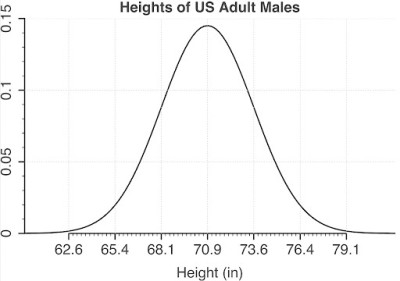
The mean of the data is 70.9 inches and the standard deviation is 2.75 inches.

Notice that the data is symmetric about the center. In normal distributions, both the mean and the median are the same. Here, the mean height of an adult male in the US will be at the peak of the normal curve, 70.9 inches. It should make sense that all of our probabilities are nonnegative. Even though the tails of the curve in both directions continue on, the area under the curve is equal to 1.

With continuous probability distributions, it’s common to ask questions about a range of values, rather than a specific number. In a continuous probability distribution, the probability that the random variable can take on an exact value is 0.

Example: A Continuous Probability Distribution

Using the graph, what is the probability that a randomly selected male from the United States has a height between 73 and 76 inches? In other words, we need to solve the inequality:

• 73 <= P(X) <= 76

Relating this to calculus, this is equivalent to finding the area under the normal curve from 73 to 76. As we hopefully remember from calculus, this is equal to the definite integral:

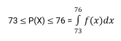
where f(x) is the function representing the normal curve in our graph. 

We don’t actually have an equation for the function f(x). But, we can use our TI-84 Plus to figure this out!

We’ll use the “normcdf” function. This stands for the normal cumulative distribution function.

This function will allow us to find the probability that our random variable will fall within the interval we supply.

In this case, we’ll calculate the probability that our variable is between 73 and 76 inches. In essence, we’ll be calculating the area under the normal curve between these two values.

Steps:

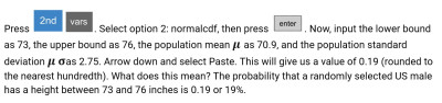
Using the same table, let’s answer the question, what is the probability that a randomly selected male is over 74 inches tall? Essentially, we need to solve:

• P(X) >= 74

To answer this question, we can once again use the normaldcf function on our calculator. In this case, we don’t have an upper bound, but we can enter a very large number as the upper bound.

Enter the lower bound as 74 and the upper bound as 9,999 (or some other very large number). The population mean and the standard deviation remain the same: 70.9 and 2.75, respectively.

Arrow down to  Paste and we get 0.13, rounded to the nearest hundredth. Hence, the probability that a randomly selected US male is over 74 inches tall is 0.13 or 13%. Cool. 

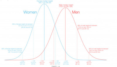
Just for fun – here is an overlay of female heights and male heights. Both sets of data are normally distributed. This data was taken from 20 countries in North America, Europe, Asia and Australia.

In addition to normal distributions, other examples of continuous probability distributions are the t-distribution, the F-distribution, and the Chi-Square distribution.

Now that we’ve had an overview of probability distributions, hopefully we’ll be better equipped to process all the data around us!

---