Exponential Decay (5 Common Questions Answered)

Exponential decay often comes up in science and math courses, including calculus.  It helps to know what this concept means and how to solve these types of problems.

So, what is exponential decay?  Exponential decay means that a number decreases by a fixed percentage in each time period. For example, exponential decay of 10% per year for a starting value of 1,000 means the value is 900 at the end of year 1, 810 at the end of year 2, 729 at the end of year 3, and so forth.

Of course, we can solve for various numbers in an exponential decay problem, including time, starting amount, ending amount, and decay rate (as a percentage).

In this article, we’ll talk about exponential decay and what it means.  We’ll also look at some examples and show how to solve them.

Let’s get started.

What Is Exponential Decay?

Exponential decay means that a quantity gets smaller over time, decreasing by a fixed percentage in each time period (the time periods all have the same duration – for example, 1 day, 1 month, or 1 year).

More specifically, we have a decay rate R (as a percentage) that tells us how much the number decays in each time period.  R is also called the exponential decay constant (when used with a base of e).

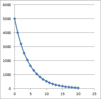
For example, an exponential decay rate of R =  20% per year for a starting value of 5,000 means:

• In the 1st year, the value decreases by 1,000 (20% of 5,000), going from 5,000 to 4,000.
• In the 2nd year, the value decreases by 800 (20% of 4,000), going from 4,000 to 3,200.
• In the 3rd year, the value decreases by 640 (20% of 3,200), going from 3,200 to 2,560.
• In the 4th year, the value decreases by 512 (20% of 2,560), going from 2,560 to 2,048.
• and so on.

Note that although the quantity remaining decreases by the same percentage in each time interval (20%), it decreases by smaller amounts in each interval (first a decrease of 1,000, followed by a decrease of 800, then 640, 512, etc.)

This is because there is less remaining after each year passes, so 20% of the remaining amount is a smaller number each year.  The following table illustrates this:

Year	Start Amount	End Amount	Decrease
1	5000	4000	1000
2	4000	3200	800
3	3200	2560	640
4	2560	2048	512
5	2048	1638	410

Also, the graph below shows exponential decay from the above example, modeled over 20 years:

Note that we can also write an equation for exponential decay:

• Q(T) = Q₀(1 – R)^T

where

• T= the time that has passed (usually we start at T = 0)
• R = the rate of decay, usually expressed as a percentage (that is, the exponential decay constant)
• Q(t) = the quantity (amount remaining) at time T
• Q₀ = Q(0) = the quantity at time t = 0 (that is, the initial quantity or starting amount)

For the example above, our starting amount was Q₀ = 5,000 and the rate of decay R was R = 0.20 (20% per year), so our equation would be:

• Q(T) = 5,000(1 – 0.2)^T
• Q(T) = 5,000(0.8)^T

So, we can use an exponential function to model exponential decay.

Does Exponential Decay Reach Zero?

As you can see from the graphs below, exponential decay approaches zero, but it never actually reaches it.  (We say that the graph of an exponential decay function has a horizontal asymptote at y = 0).

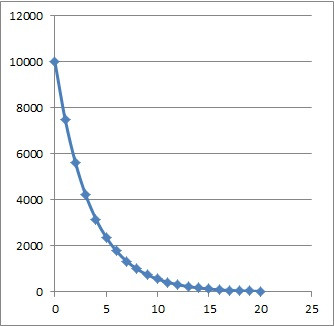
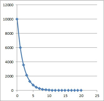
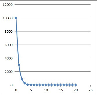
No matter the starting amount Q₀ or the rate of decay R, the graphs all have the same basic shape – they start off with a steep slope with their initial decline, and then taper off to a flatter decline as time goes by.

How To Graph Exponential Decay

To graph exponential decay from the formula, all we need to do is to pick a few times (values of T) and plug them in to the formula.  Then, we can graph the points we get and sketch an exponential decay curve to connect the dots.

Let’s look at an example to see how it works.

Example: Graphing Exponential Decay

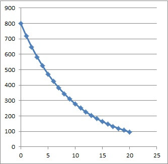
Let’s say that you start with a population of 800 people in a town.  Over time, people leave town at a rate of 10% per year.

So, our exponential decay formula has Q₀ = 800 and R = 0.10, and it looks like this:

• Q(T) = 800(0.9)^T

Let’s choose the following values of T to plug in:

• T = 0 gives us Q(0) = 800 (we can read this right from the function, since Q₀ = 800).
• T = 1 gives us Q(1) =  800(0.9)¹ = 720
• T = 2 gives us Q(2) =  800(0.9)² = 648
• T = 20 gives us Q(20) 800(0.9)²⁰ ~ 97.26

So, the first three points for us to graph are (0, 800), (1, 720), and (2, 648):

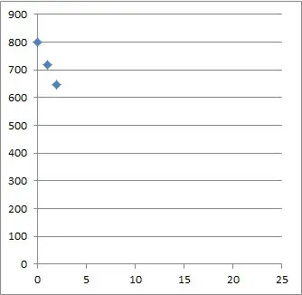
After plotting these three points, we can connect them by sketching an exponential decay curve, as shown below:

Examples Of Exponential Decay

Examples of exponential decay include:

• Depopulation
• Depreciation (cars, houses, equipment)
• Radioactive material (including half-life, or the time it takes for the mass to decrease by 50%)

Let’s look at how to solve some examples like the ones mentioned here.

How To Solve Exponential Decay Problems

To solve an exponential decay problem, there will be 3 basic steps:

• Step 1: Identify the values from the equation that we have (we should have 3 out of 4 of: T, R, Q₀, and Q(T)).
• Step 2: Write out the equation Q(T) = Q_o(1 – R)^T and plug in the known values.
• Step 3: Solve for the unknown value using algebra.

Let’s take a look at some examples to see how it works in practice.

Example 1: Exponential Decay Of Population (Depopulation)

Let’s say that you start with a population of 4,000 people in a town.  Over time, people leave town at a rate of 20% per year.

When does the town only have 2,048 people left?

Step 1: our exponential decay formula has values Q₀ = 4,000 (starting value for the population) and R = 0.20 (decay rate of 20% expressed as a decimal), and Q(T) = 2,048 (population remaining after some unknown time T).

Step 2: we write out our exponential decay equation:

• Q(T) = Q_o(1 – R)^T

and then plug in our known values:

• 2,048 = 4,000(1 – 0.2)^T
• 2,048 = 4,000(0.8)^T

Step 3: now we just need to use some algebra to solve for the value of T:

• 2,048 = 4,000(0.8)^T
• 2,048/4,000 = (0.8)^T
• log(2,048/4,000) = log(0.8)^T
• log(2,048/4,000) = Tlog(0.8)
• log(2,048/4,000) / log(0.8) = T
• 3 = T

So, the town will have 2,048 people left after 3 years (so, it takes just over 3 years for the population to decrease by half).

This means that:

• At a little over 6 years, the population will be at 25% of the original (~1,000 people)
• At a little over 9 years, the population will be at 12.5% of the original (~500 people)
• At a little over 12 years, the population will be at 6.25% of the original (~250 people)
• And so on.

Example 2: Exponential Decay Of Value (Depreciation)

Let’s say that you buy a new car that has a value of $40,000.  Over time, the value of the car decrease at a rate of 10% per year.

When is the car only worth $26,244?

Step 1: our exponential decay formula has values Q₀ = 40,000 (starting value of the car) and R = 0.10 (decay rate of 10% expressed as a decimal), and Q(T) = $26,244  (value of the car after some unknown time T).

Step 2: we write out our exponential decay equation:

• Q(T) = Q_o(1 – R)^T

and then plug in our known values:

• $26,244 = $40,000(1 – 0.1)^T
• $26,244 = $40,000(0.9)^T

Step 3: now we just need to use some algebra to solve for the value of T:

• $26,244 = $40,000(0.9)^T
• $26,244/$40,000 = 0.9^T
• log($26,244/$40,000) = log(0.9^T)
• log($26,244/$40,000) = Tlog(0.9)
• log($26,244/$40,000) / log(0.9) = T
• 4 = T

So, the car’s value will decline from $40,000 to $26,244 over the first 4 years of ownership.

We can also easily figure out what the car will be worth after T = 10 years:

• Q(T) = Q_o(1 – R)^T
• Q(10) = $40,000(1 – 0.1)¹⁰
• Q(10) = $40,000(0.9)¹⁰
• Q(10) = $40,000(0.9)¹⁰
• Q(10) ~ $13,947.14

So the value of the car is about $13,497.14 after 10 years of ownership.

After that, the car will only lose about $1,394.71 of value in the 11^th year (compare this to the $4,000 of value lost in the first year!)

Example 3: Exponential Decay Of Mass (Radioactive Decay)

The half-life of uranium-235 is 700 million years.  How long does it take for 100 grams to decay to 25 grams?

“Half-life” means the time that it takes the original mass (Q₀) to decay to half of its original amount.  So, it takes 700 million years for the initial 100 grams to decay to a mass of 50 grams.

It takes another 700 million years for the remaining 50 grams to decay to a mass of 25 grams.

In total, it takes 700 million + 700 million = 1.4 billion years for 100 grams of Uranium-235 to decay to a mass of 25 grams.

Note: we could also use the formula from before to find the time T:

• Q(T) = Q_o(1 – R)^T
• 25 = 100(0.5)^T
• 25/100 = (0.5)^T
• ¼ = (1/2)^T
• ¼ = 1/2^T
• 4 = 2^T
• 2 = T

This means that it takes 2 half-lives, or 2*700 million = 1.4 billion years for the 100 grams of Uranium-235 to decay to a mass of 25 grams.

Conclusion

Now you know what exponential decay is and what it looks like on a graph.  You also know how to solve these types of problems for each of the key parameters.

You can learn about exponential growth here.

---