
You have a big standardized exam on Saturday, but you’re not prepared. Suppose you decide that you’re going to randomly guess on every problem on this multiple choice exam.
You didn’t study and you figure, “Hey, maybe I’ll be really lucky and guess correctly on most or all of the questions!” If we think about this, for each question, even though there may be 4 or 5 answer choices, there are only 2 different outcomes: a correct answer and an incorrect answer.
This type of situation comes up frequently in statistics. And that’s what we’ll be learning about today.
Let’s get started!

In statistics, a Bernoulli trial is a random experiment in which there are two possible outcomes: success or failure. The probability of success or failure is the same each time the experiment is conducted.
Success and failure do not mean what they typically do; that is, a success isn’t necessarily a good thing, and a failure isn’t necessarily a bad thing. In statistics, success is defined as a particular outcome.
In practice, it’s typical to denote the probability of a success with the variable p and the probability of a failure with the variable q. Because there are only two possible outcomes, it follows that the probability of a failure q is equal to 1 – p.
Examples of Bernoulli Trials
- Flipping a coin is probably the first example that comes to mind when considering Bernoulli Trials. It’s the classic example because of the very nature of the experiment – we naturally get two outcomes when flipping a coin – heads or tails! Suppose flipping heads is defined to be a success. Then, p = ½ and q = ½.
- A game is designed in such a way that the player rolls a die once. If the player rolls a 6, the player wins a prize. If the player rolls anything else, they win nothing! In this case, a roll of 6 is defined as a success and any other roll (1, 2, 3, 4, or 5) is defined as a failure. Here, the probability of a success p is ⅙ and the probability of a failure q is ⅚.
- A factory produces large amounts of batteries daily. The probability of a defective battery is defined to be a success. (Strange, right? Again, a “success” isn’t what we typically think of as success – in this case, it represents a battery that doesn’t work!) A working battery is defined to be a failure. Quality assurance employees may be interested in the probability of selecting a defective battery from a group of batteries.

What are the conditions for a Bernoulli Trial?
Now that we’ve seen some examples of Bernoulli Trials, let’s formalize the conditions:
- There are only two possible outcomes for each trial. In general, we’re interested in the number of successes.
- The probability of a success is the same for each trial.
- The results are independent of one another. That is, the result of one Bernoulli Trial has no influence on the results of subsequent Bernoulli Trials.
What is the Binomial Distribution?
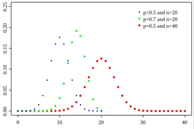
Suppose we repeat the number of Bernoulli Trials for some value of n. The Binomial Distribution represents the number of successes and failures in n independent, repeated Bernoulli Trials, each with the probability of success p.
The Bernoulli Distribution is a discrete probability distribution – it’s not continuous like the Normal Distribution.
To use the Binomial Distribution in Statistics – we first need a formula. The probability that there are r successes out of n trials is given by:
The Binomial Distribution Formula
| P(X = r) = nCr pr(1 – p)n – r where: n is the total number of trials r is the number of successes p is the probability of a success 1 – p is the probability of a failure Note: we can also write the formula using the variable q to represent the probability of a failure. Again, q = 1 – p. P(X = r) = nCr pr(q)n – r |
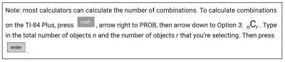
Reminder: nCr is the number of combinations of selecting subsets of size r from a set of n objects. The formula is:
- nCr = n!/r!(n – r)!
Example
A fair coin is tossed 8 times. Find the probability of obtaining:
- a. Exactly 6 heads.
- b. At least 6 heads.

Solution
Part a)
Notice that we are tossing a coin a certain number of times – the tossing of a coin is a Bernoulli Trial. When tossing the coin 8 times, to determine the probability that we obtain exactly 6 heads, we can use the Binomial Distribution formula.
Let’s identify the variables:
- n = 8 trials
- r = 6 successes
- p = ½, the probability of tossing heads
- q = 1 – ½ = ½, the probability of tossing tails
Plugging into the formula, we obtain:
- P(X = 6) = 8C6 (½)6(½)2
So we have:
- P(X = 6) = 8C6 (½)6(½)2
- =(28)(0.015625)(0.25)
- =0.109375
Therefore, the probability of obtaining exactly 6 heads on 8 tosses of a fair coin is approximately 0.109 or 10.9%. Not super likely!
Part b)
To determine the probability of flipping at least 6 heads, remember this means we need to find the probability of obtaining 6 heads, 7 heads, or 8 heads. We already calculated the probability of exactly 6 heads in part a) so now we just need to find the probability of 7 heads and 8 heads.
- P(6 heads) = 0.109 (from part a)
- P(7 heads) = 8C7 (½)7(½)1 = 0.03125 ~ 0.031
- P(8 heads)= 8C8 (½)8(½)0 = 0.00390625 ~ 0.004
Now, we add the probabilities to determine the probability of at flipping at least 6 heads:
- P(6 heads) + P(7 heads) + P(8 heads) = 0.109 + 0.031 + 0.004 = 0.144
Hence, for 8 coin flips, the probability of obtaining at least 6 heads is equal to 0.144 or 1.44%.
| Just for Fun Here is a handy calculator for computing probabilities using the Binomial Distribution: Binomial Distribution Calculator |

A common type of binomial distribution problem has to do with the number of defective items in a lot.
Example
At ABC Light Bulb Factory, it is known that the probability of a defective light bulb is always 0.015. A quality assurance employee randomly selects 20 light bulbs from the factory. Find the following probabilities:
- a. The probability that exactly 5 of the 20 bulbs are defective.
- b. The probability that at least one of the 20 bulbs is defective.
Solution
First, notice that each selection of a light bulb is independent – the probability of a defective bulb is always 0.015 and selecting one defective bulb is independent of selecting another defective bulb.
For each light bulb selected, there are only two possible outcomes – defective, which we’ll define as a success, and working, which we’ll define as a failure.
This situation meets the conditions for Bernoulli Trials. So, we can use our formula for the Binomial Distribution.
a.
P(X = r) = nCr pr(q)n – r
Define the variables:
- n = 20, the total number of light bulbs selected
- r = 5, the number of successes (defective bulbs)
- p = 0.015, the probability of success
- q = 1 – 0.015 = 0.985, the probability of failure (which in this case means a light bulb that actually lights up!)
Plug in the values:
- P(X = 5) = 20C5 (0.015)5(0.985)15
- = 0.000009385
The probability of obtaining 5 defective light bulbs out of 20 is very unlikely – practically 0. That’s good news for the factory.
b.
Finding the probability of at least one defective light bulb is pretty long and complicated to calculate directly.
We’re selecting 20 light bulbs, so “at least one defective bulb” means 1 defective bulb or 2 defective bulbs or 3 defective bulbs…all the way up to 20 defective bulbs.
That would be a LOT of calculations since we’d have to calculate each of those probabilities separately! Instead, we can use the complement of this event.
Recall that the complement of an event is all other outcomes that are not the defined event. The complement of “at least one defective bulb” is zero defective bulbs! The probability of an event and its complement must add to 1.
The Complement Rule
| Given Event A and its Complement A’: P(A) + P(A’) = 1 |
Now, we can easily calculate the probability of at least one defective bulb by using the Complement Rule!
Let’s first calculate P(zero defective bulbs).
- P(X = 0) = 20C0 (0.015)0(0.985)20
- = (0.985)20
- = 0.739136
Now, we can use the Complement Rule to determine the desired probability.
- P(at least one defective bulb)
- = 1 – P(no defective bulbs)
- = 1 – (0.985)20
- = 1 – 0.739136
- = 0.260864
Therefore, the probability of obtaining at least one defective bulb from a lot of 20 bulbs is 0.26 or approximately 26%. That’s not so good!
Let’s get back to the idea of guessing on a standardized exam question. My son recently asked about the odds of guessing correctly on most or all of the multiple choice questions on the SAT or ACT.
The ACT math section has 60 multiple choice questions, each with 5 choices. Therefore, if we’re randomly guessing on every question, the probability of a correct answer is ⅕ or 0.2.
This idea once again fits a Bernoulli Trial model – there are two possible outcomes: correct or incorrect, each guess is independent of the next guess, and the probability of a success, in this case a correct answer, is the same for every trial: p = 0.2.
Using the formula, the probability of guessing 60 out of 60 questions correctly is:
- P(X = 60)
- = 60C60 (0.2)60(0.8)0
- = 1.1529 x 10-42 0
So, the probability of guessing 60 out of 60 questions correct on the math ACT is essentially 0.
Okay wait, what if we were only hoping to get about 75% of the questions correct by guessing? What are the chances that we can obtain correct answers on 75% of the 60 questions on the math ACT?
If we want to obtain 75% of 60 questions correct this means we will need (0.75)(60) = 45 correct answers. Let’s calculate the probability of guessing 45 answers correctly.
The only value that has changed in this calculation compared with our previous calculation is r, the number of successes. In this situation r = 45.
- P(X = 45)
- = 60C45 (0.2)45(0.8)15
- = 6.585109 x 10⁻²⁰ 0
This confirms it – don’t guess randomly on a standardized test! It’s NOT a good strategy!
Connection to the Normal Distribution
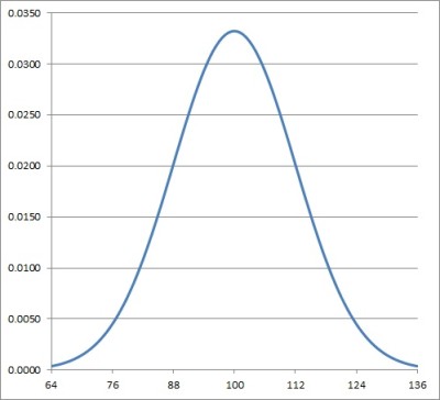
So, an interesting connection can be made between the Binomial Distribution and the Normal Distribution.
First, remember that the Binomial Distribution is a discrete distribution and the Normal Distribution is continuous. But for sufficiently large values of n with the Binomial Distribution, we can use the Normal Distribution to approximate probabilities that fit a Binomial Distribution.
For more information on this, check out this link: Normal Approximation to the Binomial Distribution.
Also, learn more about the Central Limit Theorem here.
After today’s lesson, you may think of rolling dice or flipping coins in a whole new way!
I hope you found this article helpful. If so, please share it with someone who can use the information.

Don’t forget to subscribe to our YouTube channel & get updates on new math videos!
About the author:
Jean-Marie Gard is an independent math teacher and tutor based in Massachusetts. You can get in touch with Jean-Marie at https://testpreptoday.com/.