Z-scores: What Are They Good For? (4 Great Examples)

The normal curve, sometimes called a bell curve, is a distribution of data that naturally occurs in many different situations. Lots of different types of data take on the shape of a normal curve. For example, the heights of women in the United States are normally distributed. 

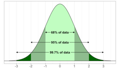
The Standard Normal Curve, shown above, is a distribution where the mean is set to 0 and the standard deviation 𝜎 is set to 1. The empirical rule, also known as the 68 – 95 – 99.7 rule, tells us what percent of data falls within a certain range for normally distributed data.

In the graph above, the shaded regions represent the data that falls within 1𝜎 of the mean, within 2𝜎 of the mean, and within 3𝜎 of the mean. Observe that nearly all of the data falls within 3 standard deviations!

To be more specific, the 68 -95 – 99.7 rule tells us that for normally distributed data:

• 68% of the data falls within 1 standard deviation of the mean
• 95% of the data falls within 2 standard deviations of the mean
• 99.7% of the data falls within 3 standard deviations of the mean

The 68 – 95 – 99.7 rule is helpful because it provides us with a tool to analyze data. For example, if we know a particular value in a data set is 3 standard deviations above the mean, we can say that result is unusual since 99.7% of the data must be within 3 standard deviations of the mean.

Similarly, if a particular value in a data set is 0.5 standard deviations below the mean, then that data value is not unusual at all since it falls within the 68% region of the normal curve. This would fall in the average range. 

(Source: statisticshowto.com)

Here’s the thing – most normally distributed data don’t have a mean equal to 0 and a standard deviation equal to 1. What do we do about that? That’s where the z-score comes in!

A z-score tells us how many standard deviations a data value is above or below the mean. And that’s the topic for this article! 

Formula for the z-score for a data set z = (x – μ)/σ where: z  =  z-score x = the observed value μ = the mean σ = the standard deviation

We can use the z-score to figure out how likely or how unusual an event is. Let’s look at several examples.

Example

Heights of women in the United State are approximately normally distributed with a mean of 64.5 inches and a standard deviation of 2.5 inches. Suppose Terry is 73 inches tall. How unusual is this for a woman in the United States? (Source: tasks.illustrative mathematics.org)

Solution

To find the z-score, let’s identify the key components in the problem. The observed value x is 73 inches, the mean is 64.5 inches and the standard deviation is 2.5 inches. Using the formula for z-score, we obtain:

z = (x – μ)/σ

= (73 – 64.5) / 2.5

 = 3.4

Terry’s height is greater than 3 standard deviations above the mean. Using the normal curve, we see that less than 0.3% of the heights of females are 3 standard deviations above or below the mean.

We know this because 99.7% of the data falls within 3 standard devotions so 100 – 99.7 = 0.3% of the data must lie outside 3 standard deviations. We can conclude that for an American woman, Terry is unusually tall! ◾

Example

(Sources: online.stat.psu.edu and act.org)

Daniel took both the SAT and the ACT, standardized tests to measure college preparedness. The tests use different scales and Daniel wants to determine which of his math scores is better.

Both exams have normally distributed scores. For the particular exams that Daniel took, the SAT math exam had a mean of 500 and a standard deviation of 100. The ACT math exam had a mean of 19.9 and a standard deviation of 5.7.

Daniel scored 630 on SAT math and 28 on ACT math. Which score is better?

Solution 

It seems like we’re comparing apples and oranges! Since the two exams use different scales, it would be pretty difficult to compare the results without the use of some statistics. Let’s calculate the z-scores for both of Daniel’s test scores and compare them. 

SAT score

Daniel’s math score x is 630, the mean is 500 and the standard deviation is 100. Using the formula for z-score, we obtain:

z = (x – μ)/σ

z = (630 – 500) / 100

z = 130 / 100

z = 1.3

Daniel’s SAT math score was 1.3 standard deviations above the mean.

ACT score:

Daniel’s math score x is 28, the mean is 19.9, and the standard deviation is 5.7. Using the formula for z-score, we obtain:

z = (x – μ)/σ

z = (28 – 19.9) / 5.7

z = 1.42

Daniel’s ACT score is 1.42 standard deviations above the mean.

Remember, the z-score tells us how far away a value is from the mean. In the case of test scores, the greater the z-score, the better the result. Since Daniel’s ACT math z-score is higher than the SAT math z-score, his ACT score is a more impressive result. ◾

Example

Suppose Daniel decides to take the ACT exam again. His goal is to perform better on the ACT math section than 97.5% of test takers. Assuming that the mean and standard deviation of this math exam are the same as before, what is the corresponding z-score he needs to reach his goal and what score does he need to obtain on the ACT?

Solution

It’s helpful to divide up our normal curve with the corresponding percentages in each section.

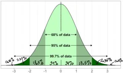
If we add all the percentages that are to the left of 2 standard deviations, we’ll see that they will add to 97.5%. So, Daniel needs to have a z-score of at least 2 in order to attain his goal. We can calculate the score x he needs to earn by using our formula:

z = (x – μ)/σ

2 = (x – 19.9) / 5.7

11.4 = x-19.9

31.3 = x

Daniel needs to have a score of at least 31.3 points on the math ACT section in order to reach his goal. Since the ACT scores are reported in whole numbers. Daniel will have to attain a score of 32. ◾

Example

Jackie and Olivia are competitive athletes. They are both on the track team but compete in different events. At a recent meet, Jackie finished the 100-yard dash with a time of 10.7 seconds where the overall mean was 11.5 seconds and the standard deviation was 0.4 seconds. Olivia ran the one mile in 6.2 minutes where the overall mean was 7.1 minutes and the standard deviation was 0.5 minutes. Who performed better in the track meet?

Solution

To compare their performances, we need to calculate their z-scores.

Jackie:

Identify the variables. Jackie’s time x is 10.7 seconds, the mean is 11.5 seconds, and the standard deviation is 0.4 seconds. Plug into our formula.

z = (x – μ)/σ

z = (10.7 – 11.5) / 0.4

z = -2

Jackie’s time was 2 standard deviations below the mean. (In the case of a race, the lower the z-score is, the better.)

Olivia

Identify the variables. Olivia’s time x is 6.2 minutes, the mean is 7.1 minutes, and the standard deviation is 0.5 minutes. Plug into our formula.

z = (x – μ)/σ

z = (6.2 – 7.1) / 0.5

z = -1.8

Olivia’s time was 1.8 standard deviations below the mean.

Because Jackie’s z-score was lower, she performed better in her race. ◾

Hopefully, this article helped you to understand how powerful statistics can be! 

---