Parametric Equations (What They Are & How To Solve Them)

In math, we’re very used to working with equations in the form y equals something in terms of x. Sometimes, it seems that’s all we do in high school math!

We’ve learned that x is called the independent variable and y is the dependent variable since its value depends on x. These equations are called rectangular equations – the associated functions can be graphed in the xy-plane, which is called the Cartestian or rectangular coordinate system. 

Examples of rectangular equations

y = 2x-10

y=x²+3x+5

2x-5y = 10

Suddenly, students are introduced to parametric equations. These can seem a bit mysterious at first but no worries, we’ll explore all the important facts of parametric equations. Let’s get started!

What is a parametric equation?

Parametric equations introduce a third variable, called the parameter. The parameter is an independent variable of the function.

Often, the parameter is t for time. Parametric equations have a horizontal component and a vertical component.

More specifically, we can define parametric equations as follows:

If x and y are continuous functions on any interval, then the equations x=x(t) y=y(t) are parametric equations, and the variable t is called the independent parameter. Sometimes, parametric equations are referred to as plane curves.

Why do we need parametric equations? Aren’t they more complicated than rectangular equations?

It may seem that mathematicians are making our lives more complicated by introducing parametric equations. Sometimes, it’s important to know the values of x and y at a certain time.

Parametric equations give us the ability to not only see which points are graphed but also, when they are graphed. Often, a plane curve will include arrows on the graph to indicate the order in which the points were graphed. 

One big advantage of using a graphing calculator to graph parametric equations is that we can watch the graphs as they are drawn so we can see the order in which the points are graphed. 

How to graph parametric equations on Desmos

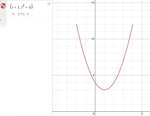
It’s pretty simple to graph parametric equations on Desmos. Simply write the parameters as an ordered pair.

For example, consider the following parametric equations.

Parametric equations for t in [-3, 3]:

x=t+1

y=t²+3

In Desmos, input the ordered pair (t+1, t²+3) and choose an interval for the variable t. In this case, we used the interval [-3, 3]. 

It’s as simple as that! Our graph in Desmos will look like this:

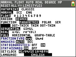
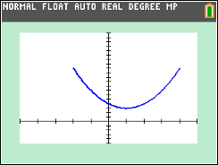
How to graph parametric equations on TI-84 Plus CE

On the TI-84 Plus CE, first, change the function mode to parametric: select [mode], scroll down to the 5th line and select PARAMETRIC. 

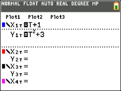
Exit out of the screen, then enter the equations into [y = ]. Notice, the calculator knows that we’ll be entering two equations. Enter X_1T = t+1 and   Y_1T = t²+3.

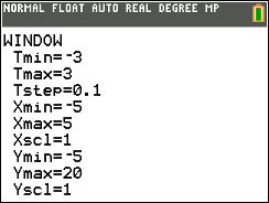
Adjust the window: choose [window] and put in the appropriate values for t: from -3 to 3, with a step of 0.1 or something similar. The smaller the t value, the more points are graphed. You can also put in appropriate minimum and maximum values for x and y. 

Finally, select [graph] and watch the order in which the function is graphed! 

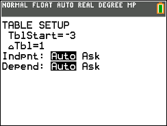
It’s also worth taking a look at a table of values. First, let’s adjust the table so that we’re looking at values of t between -3 and 3. Do this by selecting [2nd] [window], which will give us table settings.

We’ll start our t values at -3, with increments of 1 unit, so our table settings should look like this:

Now, select [2nd] [graph] to see a table of values:

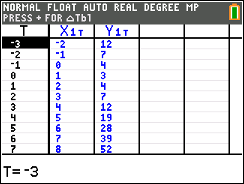
And there we have it! If we are graphing parametric equations by hand, we can do something similar – create a table of values by selecting values of t and plugging in for x and y.

Graphing parametric equations by hand

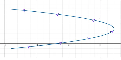
Suppose we want to graph parametric equations by hand. To do so, we can plot points over the indicated interval. We can select values for t, then calculate the values for x and y. 

Example

Sketch the graph of the parametric equations on the interval t in [-4, 4].

x=-t²+2

y=t+3

Solution

Let’s create a table using integer values of t from -4 to 4. Remember, in this case, t is the only independent variable. The variables x and y depend on t. To start, our table looks like this:

t	x	y
-4
-3
-2
-1
0
1
2
3
4

Now, we can calculate the values of x and y. Starting with t = -4, we obtain:

x=-t²+2

x=-(-4)²+2

x=-16+2

x= -14

y=t+3

y=-4+3

y=-1

Fill in the remaining parts of the first row:

t	x	y
-4	-14	-1
-3
-2
-1
0
1
2
3
4

Continuing in this manner, we can complete the table (a bit time consuming but not too difficult!)

t	x	y
-4	-14	-1
-3	-7	0
-2	-2	1
-1	1	2
0	2	3
1	1	4
2	-2	5
3	-7	6
4	-14	7

Now, plot the points in order, noting which points get plotted first. For example, looking at the first few points, we attain a graph that looks like this:

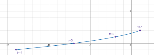
Now, finish the graph on the interval [-4, 4]. We get a horizontal parabola that opens to the left. We can put in arrows to indicate the order.  

Eliminating the parameter

Sometimes, it’s beneficial to convert parametric equations back to rectangular equations. In some cases, we may not care about the parameter so it might make sense to have rectangular equations instead. Let’s look at an example problem to see how we can do this.

x=3t+2

y=t²-7

To eliminate the parameter t, we will use the simpler equation to solve for t, then we’ll plug that expression into the other equation. In this case the simpler equation is the first one.

Solve for t:

x=3t+2

x-2=3t

x-23=t

t = x-23

Substitute this expression into the second equation:

y=t² – 7

y=((x-2)/3)² – 7

y=((x-2)²/9) – 7

y=(1/9)*(x-2)² – 7

And there we have it! We may recognize this equation as the graph of a parabola that opens up with a vertex of (2, -7).

Word problems involving parametric equations

A classic case of a word problem involving parametric equations is projectile motion. Projectile motion is the motion experienced by an object (or projectile) that is launched into the air with an initial velocity and follows a curved path subject only to the force of gravity. The path the object takes is called the trajectory. 

 Source: openstax.org

Projectile motion depends on two parametric equations: x = (v0cos θ)t y = -16t2+ (v0sinθ)t + h where v0 is the initial velocity the variable θ represents the angle at which the initial object is launched or thrown, and h is the height of the object when it is launched.

Example

In a baseball game, a home team batter hits the ball at a speed of 117 feet per second at an angle that’s approximately 32° with the horizontal. The batter makes contact with the ball 3 feet above the ground. The ball travels to left field where there’s a green wall 37 feet high. The wall is 310 feet from home plate. 

1. Where is the ball at time t = 1 second?
2. Does the ball clear the wall? In other words, is the hit a home run?

Solution

First, we’ll write the parametric equations that represent this situation. Using the models from the box above, we can identify the variables: v0=117, h=3, and  is 32°. So our parametric equations are:

x=(117 cos 32)t

y = -16t²+ (117sin32)t + 3

1. To find where the ball is at t = 1 second, we simply plug our value of t into both equations.

x=(117 cos 32)(1)

x = 99.2

y = -16t²+ (117sin32)t + 3

y = -16(1)²+ (117sin32)(1) + 3

y=49.0

            At 1 second, the ball is about 99 feet from home plate and 49 feet in the air. 

2. Since the wall is 310 feet from home plate, to figure out if the ball will clear the left field wall, we will figure out how high the ball is when x is equal to 310 feet. So, we’ll set our x equation equal to 310, solve for t, then plug that value into the y equation to see how high the ball is at that time. 

x=(117 cos 32)t

310=(117 cos 32)t

310/117cos32 = t

t = 310/117cos32 = 3.12 seconds.

Now, plug in t = 3.12 seconds into the y equation to see if the height of the ball at that time is higher than the 37 foot left field wall. 

y = -16t²+ (117sin32)t + 3

y = -16(3.12)²+ (117sin32)(3.12) + 3

y=40.7 feet. 

Indeed, this hit clears the 37 foot left field wall! It’s a home run! Go Red Sox!

Parametric equations have their uses for sure! Hopefully, this lesson helped you get a jump on parametric equations!

---