
Suppose I asked the question, what is the probability that a randomly selected teenager drinks coffee? We may think that that number is rather low. Many middle schoolers are teenagers and there probably aren’t too many coffee drinkers there – we won’t count frozen coffee drinks!

Now suppose the question were posed this way: What is the probability that a randomly selected teenager drinks coffee, given that he or she is a freshman in college?
In this case, we have a condition – we know that the teenager selected is in college. This affects the probability because now we have an added stipulation.
If we think about it a bit, it would seem that this probability is higher than it would be without the condition. Did you ever hear of a college freshman pulling an all-nighter while cramming for a big exam?
Chances are, that freshman had some coffee on hand! To answer such questions, we’ll use conditional probability, the topic of this article.
Let’s get started.
What Is Conditional Probability?
Conditional Probability is the probability that event B occurs given that event A already occurred.
The notation P(B|A) is read, “the probability of event B, given that event A occurred.” Or, more simply, P(B|A) is “the probability of event B given event A.”
Two-way Tables
To really understand conditional probabilities, it’s helpful to be familiar with two-way tables and how we can use them.
A two-way table displays frequencies of two categorical variables. The rows display one variable, and the columns display the other variable.
Example: Two-way Table
Middletown has two ice cream shops: Elliot’s Ice Cream and The Gourmet Scoop.
On one particularly hot day, 200 randomly selected people in the town center completed a survey of their ice cream preferences and their age. The results are recorded in the table below.
| Elliot’s Ice Cream | The Gourmet Scoop | TOTAL | |
|---|---|---|---|
| Age 25 and Under | 58 | 47 | 105 |
| Over 25 | 33 | 62 | 95 |
| TOTAL | 91 | 109 | 200 |
people in each of two age categories
who visited two ice cream shops.
To illustrate the difference between probability that is unconditional versus conditional probability, we’ll ask two questions:
- What is the probability that a randomly selected respondent preferred Elliot’s Ice Cream?
- What is the probability that a randomly selected respondent preferred Elliot’s Ice Cream, given that they were over 25 years of age?
Solution: First, notice the difference in the two questions.
The first question only asks about the ice cream preference probability; there is no mention of the person’s age.
The second question is asking about the likelihood that a person preferred Elliot’s Ice Cream, given the condition that they were over 25 years of age.

To answer the first question, remember:
“The probability of event A is equal to the number of favorable outcomes divided by the total number of outcomes.”
- P(A) = (Number of Favorable Outcomes) / (Total Number of Outcomes)
Working with our totals, there are 91 people who preferred Elliot’s Ice Cream over The Gourmet Scoop. Since there are 200 people that were surveyed, we have:
- P(randomly selected person prefers Elliot’s Ice Cream) = 91/200 ≈ 0.46.
To answer the second question, we need to be a little more careful. We’re now given the condition that the person who was chosen at random was over 25 so this limits the numbers with which we’ll be working.
We only want to work with the numbers in the row “Over 25.”
| Elliot’s Ice Cream | The Gourmet Scoop | TOTAL | |
|---|---|---|---|
| Age 25 and Under | 58 | 47 | 105 |
| Over 25 | 33 | 62 | 95 |
| TOTAL | 91 | 109 | 200 |
people in each of two age categories
who visited two ice cream shops.
There are a total of 95 people who are over 25. Of those, 33 preferred Elliot’s Ice Cream. So the conditional probability is:
- P(person prefers Elliot’s Ice Cream given they are over 25) = 33/95 ≈ 0.35.
Notice, the conditional probability gives us some additional insight into ice cream preferences in Midtown. It seems as though the preferences are somewhat determined by the age of the consumer. Interesting!
What is the Formula for Conditional Probability?
We’ve seen how to calculate conditional probability using two-way tables. What if we’re given some information and we want to determine the conditional probability. Is there a formula we can use? Why yes, there is!
- P(B|A) = P(A and B) / P(A)
This formula tells us that the probability of event B occurring given that event A already occurred is equal to the probability of events A and B occurring, divided by the probability of event A occurring. Let’s look at an example.
Example 1: Conditional Probability
Suppose there are 150 sophomores at Bedford Academy. Forty-five sophomores take Spanish, 60 take French and 15 take both Spanish and French. A randomly selected sophomore takes French. What is the probability that they also take Spanish?
Solution:
Let’s start by labeling our events:
- S – the sophomore takes Spanish
- F – the sophomore takes French
We want to find the probability that the selected sophomore takes Spanish given that the student takes French. So, we want to calculate P(S|F).
Using the formula, we have:
- P(S|F) = P(S and F) / P(F)
To figure this out, we need to find P(S and F) as well as P(F).
- P(S and F) = 15 out of 150 = 15/150 = 0.1
- P(F) = 60 out of 150 = 60/150 = 0.4
Therefore,
- P(S|F) = 0.1 / 0.4 = 0.25
So, the probability that the randomly selected sophomore takes Spanish, given that they take French is 0.25.
Let’s look at another problem.
Example 2: Conditional Probability
Leeya randomly drew a card from a standard deck of 52 cards. Given that she drew a card that was a heart, what is the probability that it was a face card (a face card is a Jack, Queen, or King)?
Once again, we’ll start by labeling our events:
- H – the card is a heart
- F – the card is a face card
We want to find P(F|H), the probability that the card is a face card, given that it is a heart.
For this problem, we don’t have a table of data to refer to, so we’ll have to figure out some things. There are 13 hearts in a deck of cards. There are 12 face cards: 4 Jacks, 4 Queens, and 4 Kings. And, there are only 3 face cards that are hearts. So we have:
- P(H) = 13/52
- P(F and H) = 3/52
Now, let’s calculate:
- P(F|H) = P(F and H)/P(H)
- P(F|H) = (3/52) / (13/52)
- P(F|H) = 3/13
The probability that Leeya selected a face card given that it was a heart is 3/13.
What is Bayes’ Theorem?
So at this point you might be wondering, “Hey, did anyone ever prove a math theorem that will help us with conditional probability?” The answer is a resounding “Yes!”
Thomas Bayes was a minister, a statistician, and a philosopher from England. While he never published his famous theorem, another mathematician Richard Price formally presented Bayes’ findings in 1763.
Bayes’ Theorem states:
- P(A|B) = P(B|A)·P(A) / P(B) P(B) ≠ 0
where:
- P(A) is the probability that event A occurs.
- P(B) is the probability that event B occurs.
- P(A|B) is the probability that event A occurs, given that event B occurred.
- P(B|A) is the probability that event B occurs, given that event A occurred.
So, why is Bayes’ Theorem helpful? According to Investopedia, Bayes’ Theorem has some useful applications in finance. Bayes’ Theorem is used to help financial companies determine the risk of lending money to potential borrowers.
There are other useful applications of Bayes’ Theorem in medicine. Consider:
Example: Bayes’ Theorem
In a certain city in Indiana, it is known that 1 in 5,000 people have a rare blood disorder called Midi-chlorianism.
Scientists develop a medical test that is 97% accurate in detecting the disorder; that is, if a person has the disorder, the test will be positive 97% of the time.
Additionally, of those who take the medical test it is known that 0.5% test positive for the disorder.
Andy, a resident of the town, thinks he may have the disorder so he goes to an urgent care facility and tests positive for the disorder.
What is the probability that Andy actually has Midi-chlorianism, given that the medical test was positive?
Solution: We’ll make great use of Bayes’ Theorem to figure this out:
- P(A|B) = P(B|A)·P(A)/P(B)
Once again, we’ll start by labeling our events:
- A – the person has the disorder
- B – the medical test was positive
Now, let’s determine each of the probabilities on the right side of the equation for Bayes’ Theorem.
- P(A) = 1/5,000 = 0.0002
- P(B) = 0.005
- P(B|A) = 0.97 (since the test is accurate 97% of the time)
We’ll now use Bayes’ Theorem to calculate P(A/B) – the probability that Andy has the disease given that his blood test came back positive.
Let’s plug our values into the equation:
- P(A|B) = P(B|A)*P(A)/P(B)
- P(A|B) = (0.97)*(0.0002)/0.005
- P(A|B) = 0.0388 ≈ 3.9%
Okay, so these results are kind of surprising, right? The test came back positive but the probability that Andy actually has the disorder is 3.9%. So hopefully, he won’t be too worried!
How Do You Create Probability Tables in Excel?
Sometimes, instead of looking at a two-way table with actual data, it’s helpful to use relative frequency tables. A relative frequency table shows us the data in percentage form which helps when trying to compare categories.
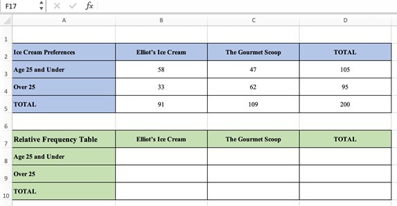
Let’s create a relative frequency table using the data from our ice cream preference example.
After copying our ice cream preference table into Excel, make another copy of the table just below it to calculate the frequencies. Change the title and the colors. We’re all set to go.
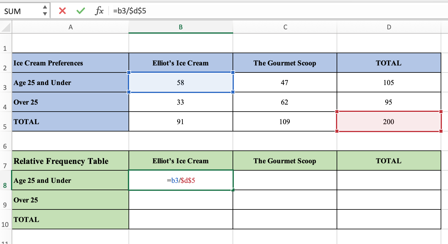
Let’s calculate the relative frequency for cell B8 – the survey respondents age 25 and under who preferred Elliot’s Ice Cream. Type the equation “=b3/$d$5.”
This will calculate 58/200. Use the $ symbol for the d and the 5 because in every case, we’ll be dividing by 200; we don’t want the spreadsheet to change that if we copy and paste the formulas.
Note, it’s very helpful to format the cells as percentages rounded to 1 decimal place, otherwise we may find our totals can be slightly off due to rounding. Once we’ve entered our first formula, we can copy and paste it to the 3 remaining cells with data. Now enter the total formulas. For example, for the first row total, enter “=SUM(b8:c8).”
After copying the formulas, Voila! We have our relative frequency table!
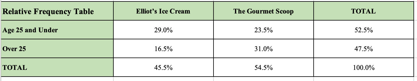
This table makes it easier to predict outcomes since we can read these cells as probabilities. Notice though that we don’t know how many people participated in the survey if we just look at the relative frequency table.
(You can also calculate mean in Excel – you can learn more here).
Conclusion
We’ve seen some good examples of how conditional probability and two-way tables can be super useful in real life. From helping us better understand the results of a medical test to accurately interpreting data from a survey, conditional probability helps us understand the relationship between two events.
You can learn more about the uses of probability here.
You can learn about the Monty Hall Problem (an example of conditional probability) here.
I hope you found this article helpful. If so, please share it with someone who can use the information.

Don’t forget to subscribe to our YouTube channel & get updates on new math videos!
About the author:
Jean-Marie Gard is an independent math teacher and tutor based in Massachusetts. You can get in touch with Jean-Marie at https://testpreptoday.com/.